cols(
  age = col_double(),
  gender = col_double(),
  city = col_double(),
  asbExposure = col_double(),
  asbDuration = col_double(),
  dxMethod = col_double(),
  cytology = col_double(),
  symDuration = col_double(),
  dyspnoea = col_double(),
  chestAche = col_double(),
  weakness = col_double(),
  smoke = col_double(),
  perfStatus = col_double(),
  WB = col_double(),
  WBC = col_double(),
  HGB = col_double(),
  PLT = col_double(),
  sedimentation = col_double(),
  LDH = col_double(),
  ALP = col_double(),
  protein = col_double(),
  albumin = col_double(),
  glucose = col_double(),
  PLD = col_double(),
  PP = col_double(),
  PA = col_double(),
  PG = col_double(),
  dead = col_double(),
  PE = col_double(),
  PTH = col_double(),
  PLA = col_double(),
  CRP = col_double(),
  dx = col_double()
)17 Logistic Regression Diagnostics and Model Selection
Things are a bit different in GLMs. There is no assumption of normality and the definition of a residual is much more ambiguous.
- We verify the linearity assumption, i.e., \(g(\mu_{y|x})\) is linearly related to the predictors. (NOT \(\mu_{y|x}\)).
- This one is a bit difficult to tease out.
- We check multicollinearty/VIF like before.
- Assess for influential observations.
17.1 Data: Do you have mesothelioma? If so call \(<ATTORNEY>\) at \(<PHONE NUMBER>\) now.
17.1.1 Data description
From UCI Machine Learning Repository: https://archive.ics.uci.edu/ml/datasets/Mesothelioma%C3%A2%E2%82%AC%E2%84%A2s+disease+data+set+
This data was prepared by; >Abdullah Cetin Tanrikulu from Dicle University, Faculty of Medicine, Department of Chest Diseases, 21100 Diyarbakir, Turkey e-mail:cetintanrikulu ‘@’ hotmail.com Orhan Er from Bozok University, Faculty of Engineering, Department of Electrical and Electronics Eng., 66200 Yozgat, Turkey e-mail:orhan.er@bozok.edu.tr
In order to perform the research reported, the patient’s hospital reports from Dicle University, Faculty of Medicine’s were used in this work. One of the special characteristics of this diagnosis study is to use the real dataset taking from patient reports from this hospital. Three hundred and twenty-four MM patient data were diagnosed and treated. These data were investigated retrospectively and analysed files.
In the dataset, all samples have 34 features because it is more effective than other factors subsets by doctor’s guidance. These features are; age, gender, city, asbestos exposure, type of MM, duration of asbestos exposure, diagnosis method, keep side, cytology, duration of symptoms, dyspnoea, ache on chest, weakness, habit of cigarette, performance status, White Blood cell count (WBC), hemoglobin (HGB), platelet count (PLT), sedimentation, blood lactic dehydrogenise (LDH), Alkaline phosphatise (ALP), total protein, albumin, glucose, pleural lactic dehydrogenise, pleural protein, pleural albumin, pleural glucose, dead or not, pleural effusion, pleural thickness on tomography, pleural level of acidity (pH), C-reactive protein (CRP), class of diagnosis. Diagnostic tests of each patient were recorded.
17.2 Model Selection
There are a lot of variables in the data…AND I don’t have a code book for what some of the stuff means.
What do I do?
17.2.1 Step one: Assess your goal and how you get there.
The goal will be to predict the probability of the subject having mesothelioma:
dxis 1 for mesothelioma, 0 if “healthy”- I want to do this for people that are ALIVE. And I want to do it based on the characteristics of the person
- The
deadvariable is therefore useless to me, I can get rid of it. dxMethoddoesn’t seem useful for my goal by its name either.- I’m suspicious of
cytologysince it may be whether a specific type of test is used. That would not be helpful in actually predicting if someone has mesothelioma based on the attributes of that person.
- The
- There are many categorical variables that I don’t know how they are coded.
city,smoke,perfStatus- If I can’t assess how they contribute to the model, I’m not going to use them.
- I don’t know how to measure those variables for future use of the model.
- Also, as a statistician, I can’t give meaningful results if I don’t have information about a variable.
That still leaves of with 24 variables…
17.2.2 Variance Inflaction Factors are still here
Let’s start with the full model.
Now get the VIFs (courtesy of ’car library)
          age        gender   asbExposure   asbDuration   symDuration
     1.623728      1.097621      2.719456      3.482200      1.141027
     dyspnoea     chestAche      weakness            WB           WBC
     1.094622      1.062902      1.220221      1.119346      1.124898
          HGB           PLT sedimentation           LDH           ALP
     1.157734      1.886302      1.135334      1.870804      1.247170
      protein       albumin       glucose           PLD            PP
     1.336606      1.413671      1.102442      1.250738      7.939269
           PA            PG            PE           PTH           PLA
     7.117496      2.344206      2.351430      1.705495      1.878006
          CRP
     1.565218
The criteria is about the same as before:
If there are any VIFs greater than 5, investigate.
If there are more than a few (no hard rule to give) in the 2 to 5 range or things seem weird, investigate.
What strikes me is
absExposureandabsDuration.- These are whether someone has been exposed, and if so, how long were they exposed in
days. - They are NOT independent of each other.
- There are things to consider which one is wisest to remove.
asbDurationcontains information about both, so maybe that’s best.
- These are whether someone has been exposed, and if so, how long were they exposed in
That leaves us mainly with
PP(pleural protein?) andPA(pleural albumin?)- They seem to be fairly correlated with each other.
- I have no idea what is more important (maybe you would!) so I’m going to take
PPout. - A less arbitrary option may be to try two models, one with each missing, and see how well they fit/perform.
17.2.3 Check after removing variables
So lets cut the variables down a bit more and check how things are doing.
Call:
glm(formula = dx ~ ., family = binomial, data = meso3)

Coefficients:
                Estimate Std. Error z value Pr(>|z|)
(Intercept)    1.227e+00  1.944e+00   0.631  0.52779
age           -4.656e-02  1.472e-02  -3.163  0.00156 **
gender        -7.519e-01  2.735e-01  -2.749  0.00597 **
asbDuration    2.945e-02  1.059e-02   2.781  0.00541 **
symDuration    5.788e-02  2.902e-02   1.994  0.04611 *
dyspnoea      -2.021e-02  3.484e-01  -0.058  0.95375
chestAche     -2.540e-01  2.830e-01  -0.898  0.36939
weakness       3.429e-01  2.964e-01   1.157  0.24726
WB            -1.577e-05  3.982e-05  -0.396  0.69201
WBC           -6.393e-02  4.185e-02  -1.528  0.12655
HGB            3.258e-01  2.844e-01   1.146  0.25195
PLT           -2.201e-03  1.140e-03  -1.931  0.05349 .
sedimentation  4.768e-03  6.457e-03   0.738  0.46024
LDH            4.156e-04  9.604e-04   0.433  0.66522
ALP           -8.684e-04  4.290e-03  -0.202  0.83961
protein        7.299e-02  1.800e-01   0.405  0.68512
albumin        6.421e-02  2.442e-01   0.263  0.79262
glucose        2.416e-03  3.496e-03   0.691  0.48940
PLD           -1.459e-04  3.582e-04  -0.407  0.68367
PA            -2.819e-01  1.862e-01  -1.514  0.12996
PG            -8.418e-03  7.333e-03  -1.148  0.25097
PE             1.416e-01  5.414e-01   0.262  0.79366
PTH            2.249e-01  3.475e-01   0.647  0.51747
PLA           -7.894e-01  3.567e-01  -2.213  0.02689 *
CRP            1.226e-02  7.395e-03   1.658  0.09730 .
---
Signif. codes:  0 '***' 0.001 '**' 0.01 '*' 0.05 '.' 0.1 ' ' 1

(Dispersion parameter for binomial family taken to be 1)

    Null deviance: 393.79  on 323  degrees of freedom
Residual deviance: 348.20  on 299  degrees of freedom
AIC: 398.2

Number of Fisher Scoring iterations: 5
age gender asbDuration symDuration dyspnoea
1.434130 1.088232 1.487264 1.129502 1.094376
chestAche weakness WB WBC HGB
1.045581 1.178690 1.115586 1.096017 1.157860
PLT sedimentation LDH ALP protein
1.858685 1.140208 1.871628 1.230647 1.306394
albumin glucose PLD PA PG
1.344529 1.098984 1.235294 1.800686 2.337586
PE PTH PLA CRP
2.122909 1.701094 1.857195 1.558289 Everything is way better in terms of VIF so that’s a good first step I’d say.
17.3 Residual Diagnostics
17.3.1 Review
Assessing the residuals is a bit difficult here, originally it was pretty simple.
\[e_i = \text{observed} - \text{predicted} = y_i - \hat y_i\]
And then there are standardized residuals and studentized residuals (which get called standardized residuals because someone was sadistic).
\[e^*_i = \frac{y_i - \hat y_i}{\sqrt{MSE}} \qquad \text{or} \qquad e^*_i = \frac{y_i - \hat y_i}{\sqrt{MSE(1 - h_i)}}\]
- Both have the same objective: set the residuals on the same scale no matter what model you’re examining.
- Standardized/Studentized Residuals greater than 3 are considered outl;iers and the corresponding data point should be investigated.
- Studentized residuals (the right hand-side version) are calculated in such a way that they try to account for over-fitting of the model to the data by pretending that observation is not in the data.
- It is my impression (and opinion) that Studentized should be preferred.
17.3.2 Residuals in GLMs
Residuals follow the same form.
\[e_i = \text{observed} - \text{predicted} = y_i - \hat y_i\]
The general form for a standardized residual is about the same:
\[e_i = \frac{y_i - \hat y_i}{s(\hat y_i)}\]
and \(s(\hat y_i)\) is the variability of our estimate.
- In GLMs it is often the case, \(s(\hat y_i)\) is not constant by default, i.e., the variability of the predictions is not constant.
- Dependent on our model, the way to calulate \(s(\hat y_i)\) differs.
17.3.3 Pearson Residuals
We have to account for the fact that our predictions are probabiliies in logistic regression.
\[\hat y_i = \widehat P(y_i = 1| x) = \widehat p_i(x_i)\]
We are dealing with the binomial distribution so the formula for the variability of the predicted probability is:
\[s(\hat y_i) = \sqrt{\widehat p_i(x_i)(1-\widehat p_i(x_i))}\]
Therefore the Pearson standardized residual is:
\[e_i = \frac{y_i - \widehat p_i(x_i)}{\sqrt{\widehat p_i(x_i)(1-\widehat p_i(x_i))}}\]
If you can group your predictions somehow in groups of size \(n_i\), then the pearson residual is
\[e_i = \frac{y_i - \widehat p_i(x_i)}{\sqrt{n_i\widehat p_i(x_i)(1-\widehat p_i(x_i))}}\]
17.3.4 Deviance residuals
There is something called a deviance residual, for which the formula is:
\[e^*_i = sign(y_i - \hat y_i)\sqrt{2 [ y_i \log(\frac{y_i}{\hat y_i}) + (n_i-y_i) \log(\frac{n_i-y_i}{n_i -\hat y_i}) ]}\]
- The formula is not very illuminating unless you have deeper theoretical knowledge.
- I have seen at least one person say this is “preferred”.
- I have also seen that examining them is about the same as examining the pearson residuals.
- An advantage here is that deviance residuals are universal and relate to some of the deeper structure of GLMs.
17.3.5 Autoplot maybe?
We can examine the residuals via autoplot and assess outliers as well..
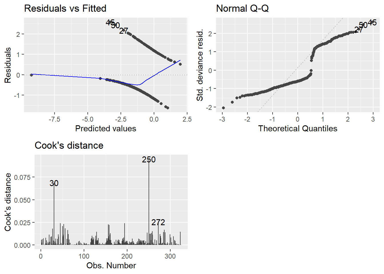
- Technically, these plots indicate that nothing is wrong.
- There is a lot of intuition and theory type stuff for why I can say that.
- That might be a whole more week’s worth of material, but we are cutting here.
- Consider it a self study topic.
- Hopefully, I’ve given enough of a seed of information for you to teach yourself more in depth modeling.
- If you want to be good, the learning never ends.
Anyway, on to the plots.
- Top-left may not be familiar since our observed values are either zero or one.
- QQ plot looks weird because there is not a normal distribution to expect, necessarily.
- Cook’s distance is at least familiar.
- 0.5 denotes a potentially problematic value.
- 1 is the cutoff for an extreme outlier.
- Some people say 4/n is a good cutoff… I have found no reason to back that up so far.
- Honestly I am still at a loss for how useful examination of the plots can be. GLMs can really mess with traditional methods.
17.3.6 DHARMa package for plotting residuals.
An experimental way of examining the residuals is availbale via the DHARMa package.
Florian Hartig (2021). DHARMa: Residual Diagnostics for Hierarchical (Multi-Level / Mixed) Regression Models. R package version 0.4.1. https://CRAN.R-project.org/package=DHARMa
- It tries to streamline the process and make it easier for non-experts to examine residuals via simulation.
- There are only a couple of functions you need to know.
simulateResiduals(model)which is stored as a variable.plot(simRes)wheresimResis the simulated residuals output variable.
- Because it runs simulations (repeated calculations), it may take a while to finish.
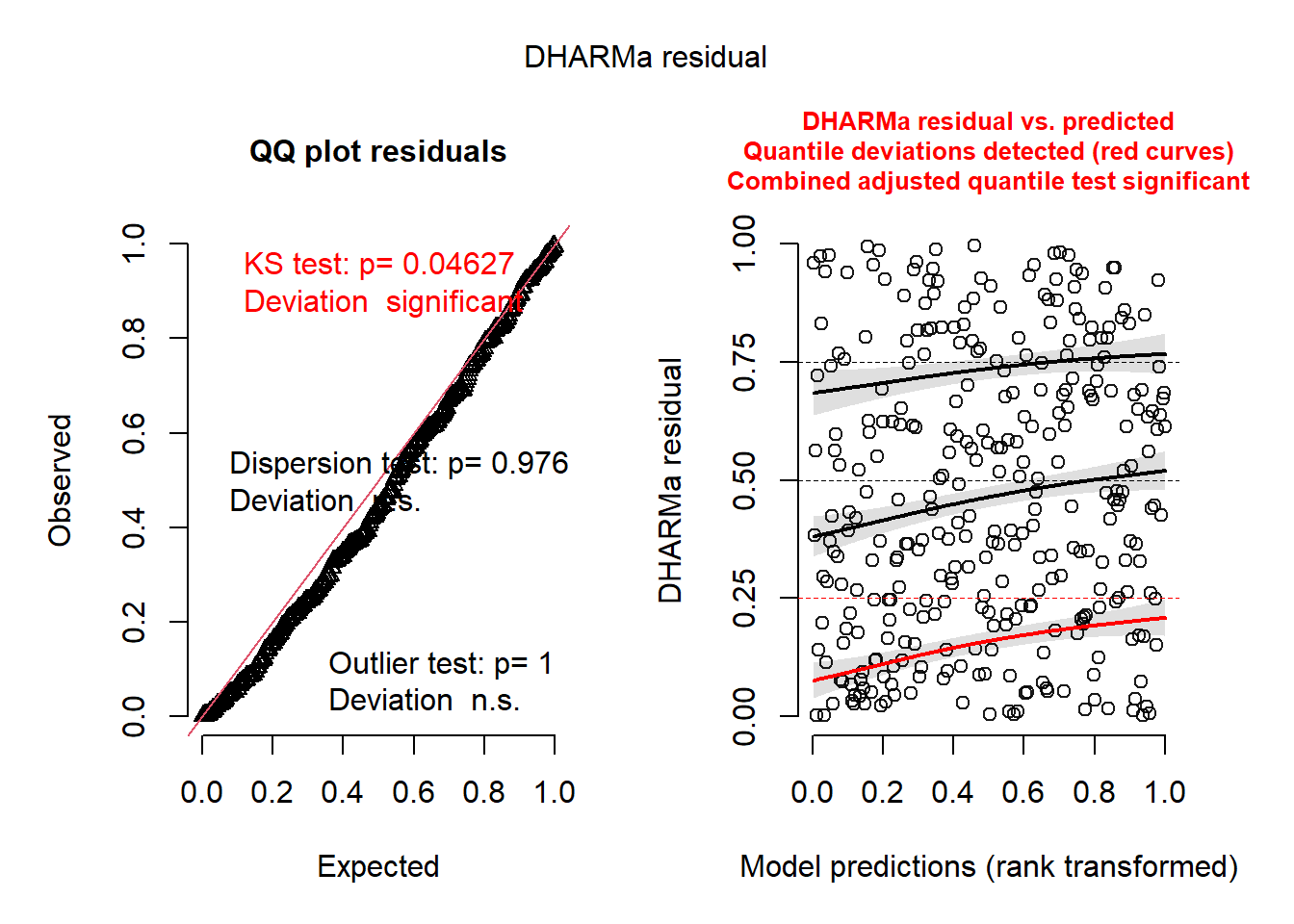
Notice the output basically tells you what may or may not be wrong. It’s as simple as that.
- The QQ Plot is NOT for normality.
- BUT you still want to check if they follow a straight line.
- The KS Test p-value is for the test of whether the data are following the correct distribution or not.
- Small p-values mean there are problems with your model.
- Here everything seems ideal.
- The QQ-Plot is a nearly straight line.
- The residual plot on the right follows the pattern we’d want. Everything is centered at 0 and the spread is consistent.
- I cannot 100% recommend that this is all that you rely on, I am merely proposing a tool to get an overview of the situation.
- In reality there are a LOT of nuances to what’s going on, so be wary.
- As far as the relative simplicity of the models we look at, my guess is that this is fine to use.
17.4 Marginal Effects
If you haven’t picked up on it yet, interpreting the logit link model is rather hard in comparison to a “normal” linear regression model.
On top of reporting the model coefficients, we should probably report the marginal effects as well.
The marginal effects are, in their most basic forms, calculations derived from the model not represented by the coefficients alone.
They take many forms.
17.4.1 What are marginal effects
Suggested Read: https://www.andrewheiss.com/blog/2022/05/20/marginalia/
Statistics is all about lines, and lines have slopes, or derivatives. These slopes represent the marginal changes in an outcome. As you move an independent/explanatory variabl, what happens to the dependent/outcome variable?
Think back to the last unit where we calculated the “marginal means” from the ANOVA using the emmeans R package. These were important because sometimes they are not equal to the summary statistics.
Marginal effect: the statistical effect for continuous explanatory variables; the partial derivative of a variable in a regression model; the effect of a single slider
Conditional effect or group contrast: the statistical effect for categorical explanatory variables; the difference in means when a condition is on vs. when it is off; the effect of a single switch
Average marginal effect vs Marginal effect at the Mean
- It matters a lot outside of normal linear regression
17.4.2 Example Data (real study)
So why do you need to know about this: interpretation.
Let’s use an example from the GUSTO study.
Let’s load the packages and study data.
| Characteristic | OR1 | 95% CI1 | p-value |
|---|---|---|---|
| tx | |||
| tPA | — | — | |
| SK | 1.24 | 1.12, 1.37 | <0.001 |
| age | 1.07 | 1.07, 1.08 | <0.001 |
| Killip Class | |||
| I | — | — | |
| II | 2.10 | 1.88, 2.35 | <0.001 |
| III | 4.70 | 3.73, 5.89 | <0.001 |
| IV | 20.8 | 15.6, 27.8 | <0.001 |
| Previous MI | |||
| no | — | — | |
| yes | 1.71 | 1.54, 1.91 | <0.001 |
| MI Location | |||
| Inferior | — | — | |
| Other | 1.36 | 1.04, 1.75 | 0.020 |
| Anterior | 1.78 | 1.62, 1.96 | <0.001 |
| Sex | |||
| male | — | — | |
| female | 1.41 | 1.27, 1.56 | <0.001 |
| 1 OR = Odds Ratio, CI = Confidence Interval | |||
So we have an effect… but what does an odds ratio really mean? Is it big or small?
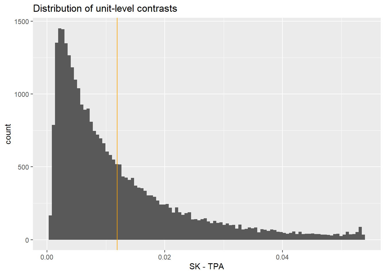
Using the marginal means, we can calculate the risk difference instead which is adjusted for the covariates. The treatment effect on this scale will vary based on the covariate values.
We can then calculate the average treatment effect on the probability (response scale) with the following:
 Estimate Std. Error    z Pr(>|z|)    S   2.5 % 97.5 %
   0.0119    0.00281 4.24   <0.001 15.5 0.00641 0.0174

Term: tx
Type:  response
Comparison: mean(SK) - mean(tPA)
Columns: term, contrast, estimate, std.error, statistic, p.value, s.value, conf.low, conf.high, predicted_lo, predicted_hi, predicted
This study, with this model, shows roughly at 1.11% reduction in risk.
We could also talk about risk in terms of relative effect. These are called risk ratios:
 Estimate Pr(>|z|)    S 2.5 % 97.5 %
     1.19   <0.001 14.7   1.1    1.3

Term: tx
Type:  response
Comparison: ln(mean(SK) / mean(tPA))
Columns: term, contrast, estimate, p.value, s.value, conf.low, conf.high, predicted_lo, predicted_hi, predicted
Shows about a 1.18 times higher risk in the SK treatment group.
17.4.3 Average Effect at the Mean
This is what you get in most software.
 Estimate Std. Error    z Pr(>|z|)    S   2.5 % 97.5 %  age Killip pmi    miloc
  0.00506     0.0012 4.22   <0.001 15.4 0.00271 0.0074 60.9      I  no Inferior
  sex
 male

Term: tx
Type:  response
Comparison: SK - tPA
Columns: rowid, term, contrast, estimate, std.error, statistic, p.value, s.value, conf.low, conf.high, predicted_lo, predicted_hi, predicted, tx, age, Killip, pmi, miloc, sex, day30
UH OH! The effect is substantially very small compared to the average effect. Why? This is for a data point that doesn’t exist!
17.4.4 Individual level summary
Again, the effect varies on individual level based on the effect of other covariates. This is more extreme when the base probability is very low (rare event).
17.4.5 What about continuous variables?
We can look at the slopes.
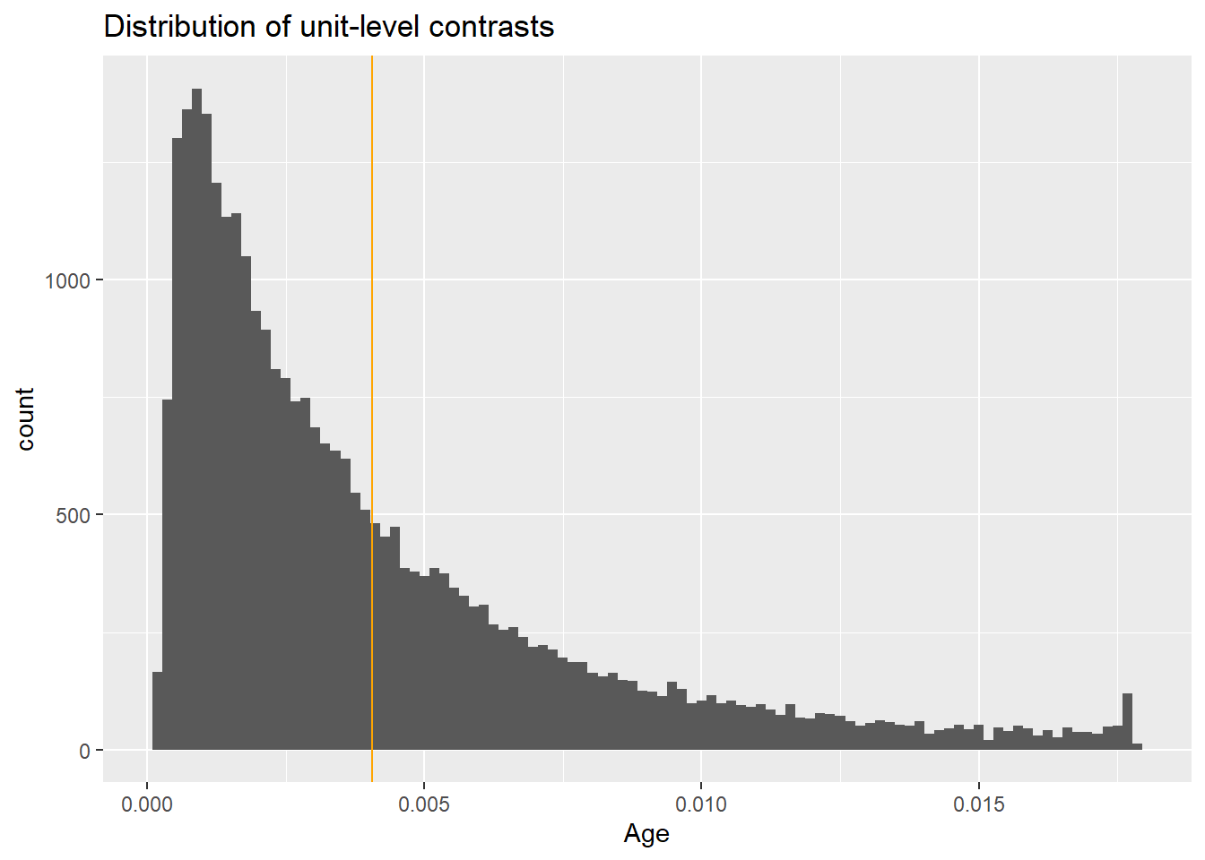
Let’s look at age!
 Estimate Std. Error    z Pr(>|z|)     S   2.5 %  97.5 %
  0.00406   0.000149 27.3   <0.001 543.6 0.00377 0.00435

Term: age
Type:  response
Comparison: mean(dY/dX)
Columns: term, contrast, estimate, std.error, statistic, p.value, s.value, conf.low, conf.high, predicted_lo, predicted_hi, predicted
So approximately at .4% increase in risk per year increase in age
Let’s plot this to see what it looks like.
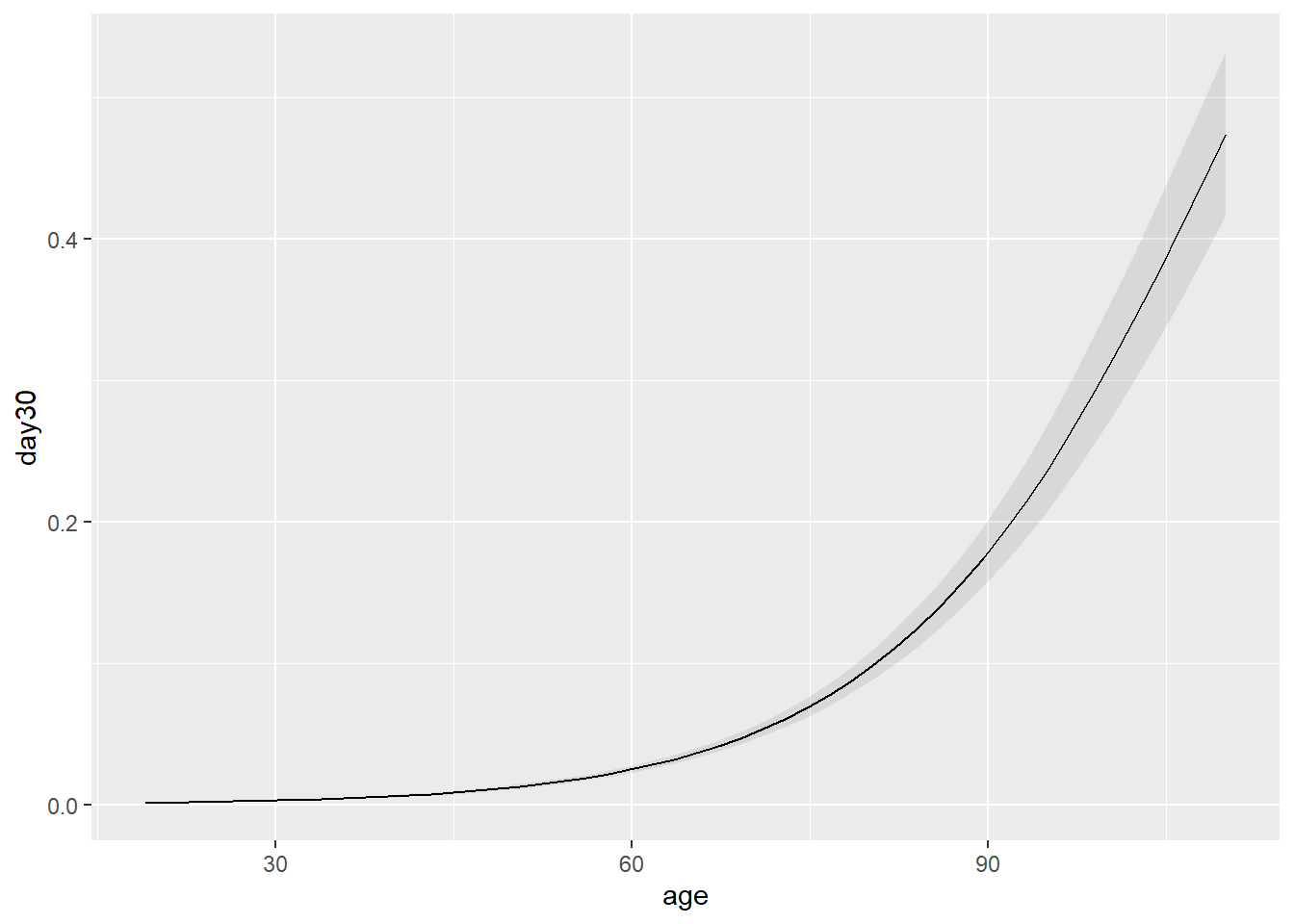
That doesn’t look linear…. Why? We model the log odds not the probability directly.
We can look at all the individual level slopes as well.