knitr::opts_chunk$set(echo = TRUE, tidy = TRUE,
                      cache = T, message = FALSE, warning = FALSE)
# Very standard packages
library(tidyverse)
library(knitr)
library(ggpubr)
library(readr)

library(ggstatsplot)
# Globally changing the default ggplot theme.

## store default
old.theme <- theme_get()

## Change it to theme_bw(); i don't like the grey background.
## Look up other themes to find your favorite!
theme_set(theme_bw())4 Simple Linear Regression
The Model, Estimating the Line, and Coefficient Inference
4.1 Statistical Models
Simple Model:
\[Y \sim N(\mu, \sigma)\]
This can be translated to:
\[Y = \mu + \epsilon\]
Where \(\epsilon \sim N(0, \sigma)\).
This second form is the basis for linear models:
- The mean of a random variable \(Y\) can be written as a linear equation which in this case would be just a flat line.
- There is an error term \(\epsilon\) that describes the deviation we expect to see from the mean.
- \(\epsilon\) having a mean of 0 means that the linear equation for the mean of \(Y\) is correctly specified.
- By correctly specified I mean that we don’t know what the actual mean of \(Y\) is, we are just crossing our fingers.
A more general model would be:
\[Y = g(x) + \epsilon\]
- \(g(x)\) represents some sort of function with an argument \(x\) which outputs some constant.
- \(g(x)\) is the deterministic portion of our model, i.e., it always gives the same output when given a single input.
- \(\epsilon\) is the random component of our model.
- The whole entire point of statistics is that there is randomness and we have to figure out how to deal with it.
- We try to distill the signal \(g(x)\) out of the noise \(\epsilon\) of chaos/randomness. (Maybe overly “poetic”)
Anyway, we try to take a stab at (guess) what the structure of \(g()\) is.
\(Y = \mu + \epsilon\) with \(\epsilon \sim N(0, \sigma)\) is about as simple of a model as we get.
We will assume from hereon that \(\epsilon \sim N(0, \sigma)\)
4.1.1 The Linear Regression Model
We assume that the mean is some linear function of some variables \(x_1\) through \(x_k\).
\[Y = \beta_0 + \sum_{i=1}^k\beta_i x_i + \epsilon\]
We will first start with the simplest linear regression model which is one that has only one input variable.
\[Y = \beta_0 + \beta_1 x + \epsilon\]
This gives us the form for how we could picture the data produced by the system we try to model.
n = 50

# Need x values
dat <- data.frame(x = rnorm(n, 33, 5))  #n, mu, sigma

# need a value for coefficients.
B <- c(300, -5)  # don't forget the y-intercept.

# Deterministic portion
dat$mu_y <- B[1] + B[2] * dat$x

# Introducing error
dat$err <- rnorm(n, 0, 20)

dat$y <- dat$mu_y + dat$err

ggplot(dat, aes(x = x, y = y)) + geom_point(data = dat, mapping = aes(x = x, y = mu_y),
    col = "red") + geom_point(data = dat, mapping = aes(x = x, y = y), col = "blue") +
    geom_segment(aes(xend = x, yend = mu_y), alpha = 0.8, col = "royalblue3") + geom_abline(intercept = B[1],
    slope = B[2]) + theme_bw()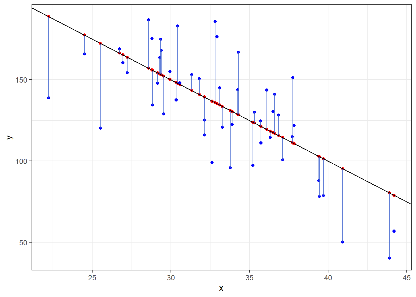
- The black line is the true mean of \(Y\) at a given value of \(x\): \(\mu_{y|x} = 300 -5x\)
- The red dots are randomly chosen points along the line.
- The blue dots are what happens when we include that error term \(\epsilon\) and shows how actual observations deviate from the line.
- Run this code a few times to see things sample to sample.
4.1.2 Comparing the Real to the Ideal
Here is data on 226 beers: ABV and Calories per 12oz.
Alcohol “contains” calories, so the more alcohol in a beer means more calories!
Assuming you have a 12 ounce mixture of water and pure alcohol (ethanol) the exact equation for the number of calories based on ABV denoted by \(x\) is
\[f(x) = 19.05x + 0\]
Let’s plot out the data on the beers and that equation.
beer <- read.csv(here::here("datasets", "beer.csv"))

ggplot(beer, aes(x = ABV, y = Calories)) + geom_point() + geom_abline(slope = 19.05,
    col = "red")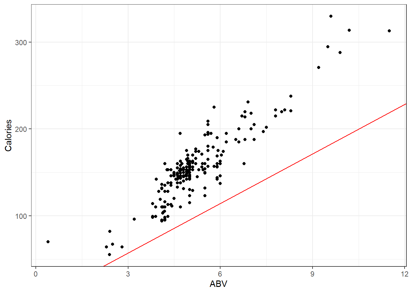
Looks like that misses the mark. I suppose there is other stuff in beer besides alcohol.
So if were to plot a line for the actual on hand, perhaps you will agree that the one in blue is a “good” one.
## OLD CODE ggplot(beer, aes(x = ABV, y = Calories)) + geom_smooth(method =
## 'lm', se = F) + geom_point() + geom_abline(slope = 19.05, col = 'red') +
## stat_cor()

# NEW CODE
ggscatterstats(data = beer, x = ABV, y = Calories, bf.message = FALSE, marginal = FALSE) +
    geom_abline(slope = 19.05, col = "red")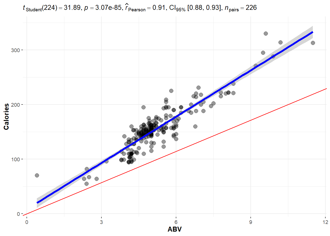
The blue line is the one we will learn how to make.
The line is meant to estimate the mean value of \(Y\):
\[\mu_{y|x} = \beta_0 + \beta_1 x\]
We have to figure out what values we should use for \(\beta_0\) and \(\beta_1\).
- \(\beta_0\) and \(\beta_1\) are the true and exact values for the intercept and slope of the line. These are unknown and are referred to as parameters of our model.
- We but ^ over the symbol for parameters to denote an estimate of the parameter.
- \(\hat \beta_0\) is our \(y\) intercept estimate.
- \(\hat \beta_i\) is our slope estimate.
- Our overall estimate for the line is \(\hat \mu_{y|x} = \hat\beta_0 + \hat\beta_i x\)
- Often we also write \(\hat y = \hat \beta_0 + \hat \beta_i x\).
Regardless, what approach(es) can we take to create \(good\) values for \(\hat\beta_0\) and \(\hat\beta_i\)?
4.2 Least Squares Regression Line
Here is a plot of the data with what is called the least squares regression line.
beerLm <- lm(Calories ~ ABV, beer)


ggplot(beer, aes(x = ABV, y = Calories)) + geom_point() + geom_smooth(method = "lm",
    se = FALSE) + geom_segment(aes(x = ABV, y = Calories, xend = ABV, yend = beerLm$fitted.values),
    alpha = 0.8, col = "royalblue3") + theme_bw()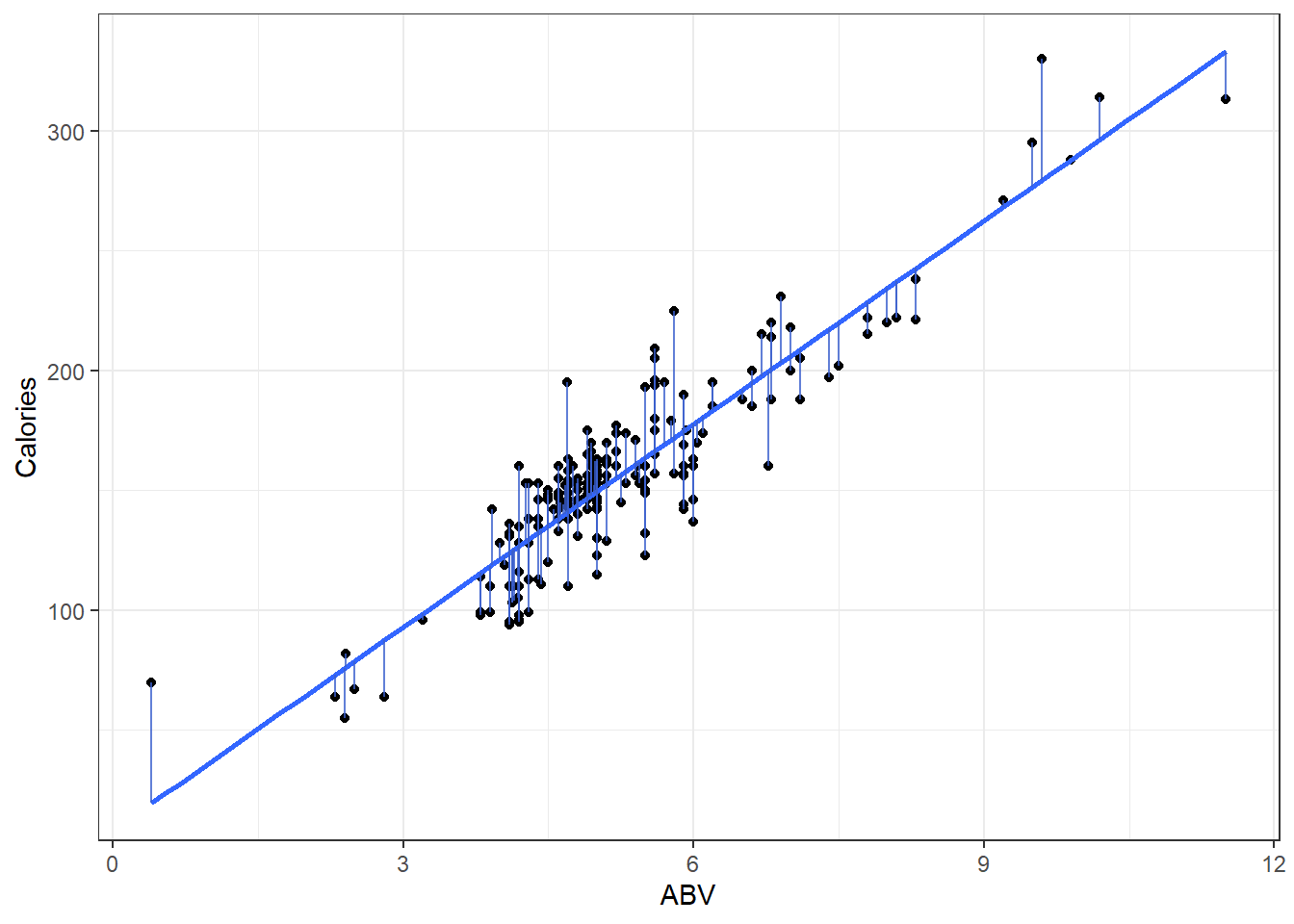
4.2.1 Measuring Error
- Sum of Squared Error
\[ SSE = \sum_{i=1}^n \left( y_i - \left(\hat \beta + \hat \beta x_i\right) \right)^2 = \sum_{i=1}^ne_i^2 \]
4.2.2 OLS solution (You can ignore this if you want.)
We want to find values of \(\hat \beta_0\) and \(\hat \beta_i\) that minimize the error sum of squares:
\[ \begin{aligned} SSE &= \sum (y - \hat{y})^2 \\ &=\sum_{i=1}^n \left( y_i - \left(\hat \beta_0 + \hat \beta_i x_i\right) \right)^2. \end{aligned} \]
To estimate to find \[ \frac{\partial}{\partial \hat \beta_i} SSE = \sum -2x(y - (\hat \beta_0 + \hat \beta_i)) = 0 \]
After substituting in our equation for \(\hat\beta_i\) above and doing quite a lot of algebra, we can make \(\hat\beta_i\) the subject.
\[ \begin{aligned} \hat\beta_i &= \frac{\sum xy - n \bar{x} \bar{y}}{\sum x^2 - n \bar{x}^2} \\ &= \frac{\sum{(x - \bar{x})(y - \bar{y})}}{\sum{(x-\bar{x})^2}} \end{aligned} \]
\[ \begin{aligned} \frac{\partial}{\partial \hat\beta_0} SSE &= \sum -2\left( y_i - \left(\hat \beta_0 + \hat \beta_i x_i\right) \right) = 0 \\ \sum \left( y_i - \left(\hat \beta_0 + \hat \beta_i x_i\right) \right) &= 0 \\ \sum y &= \sum\left( y_i - \left(\hat \beta_0 + \hat \beta_i x_i\right) \right) \\ \frac{\sum y}{n} &= \frac{\sum{\left(\hat \beta_0 + \hat \beta_i x_i\right)}}{n}\\ \bar{y} &= \hat \beta_0 + \hat \beta_i \bar{x} \end{aligned} \]
Substituting \(\bar{x}\) into the regression line gives \(\bar{y}\). In other words, the regression line goes through the point of averages.
4.2.3 Now you “know” the theory, lets look at what we do.
Okay, we’re using R. That function does regression for us? lm() !!!
Use ?lm to get a somewhat understandable summary that works pretty well once you learn how people screw up summarizing functions…
Any… Back to lm()
- there is a formula argument and a data argument. That’s all you need to know for now.
Let’s use it on that beers dataset and see what we get.
### Make an lm object

beers.lm <- lm(Calories ~ ABV, beer)

summary(beers.lm)
Call:
lm(formula = Calories ~ ABV, data = beer)

Residuals:
    Min      1Q  Median      3Q     Max
-40.738 -13.952   1.692  10.848  54.268

Coefficients:
            Estimate Std. Error t value Pr(>|t|)
(Intercept)   8.2464     4.7262   1.745   0.0824 .
ABV          28.2485     0.8857  31.893   <2e-16 ***
---
Signif. codes:  0 '***' 0.001 '**' 0.01 '*' 0.05 '.' 0.1 ' ' 1

Residual standard error: 17.48 on 224 degrees of freedom
Multiple R-squared:  0.8195,    Adjusted R-squared:  0.8187
F-statistic:  1017 on 1 and 224 DF,  p-value: < 2.2e-16
Our estimated regression line is:
\[\hat y = 8.2364 + 28.2485x\]
Or to write it as an estimated conditional mean.
\[\hat \mu_{y|x} = 8.2364 + 28.2485x\]
And that’s where we get this line:
ggplot(beer, aes(x = ABV, y = Calories)) + geom_point() + geom_smooth(method = "lm",
    se = TRUE)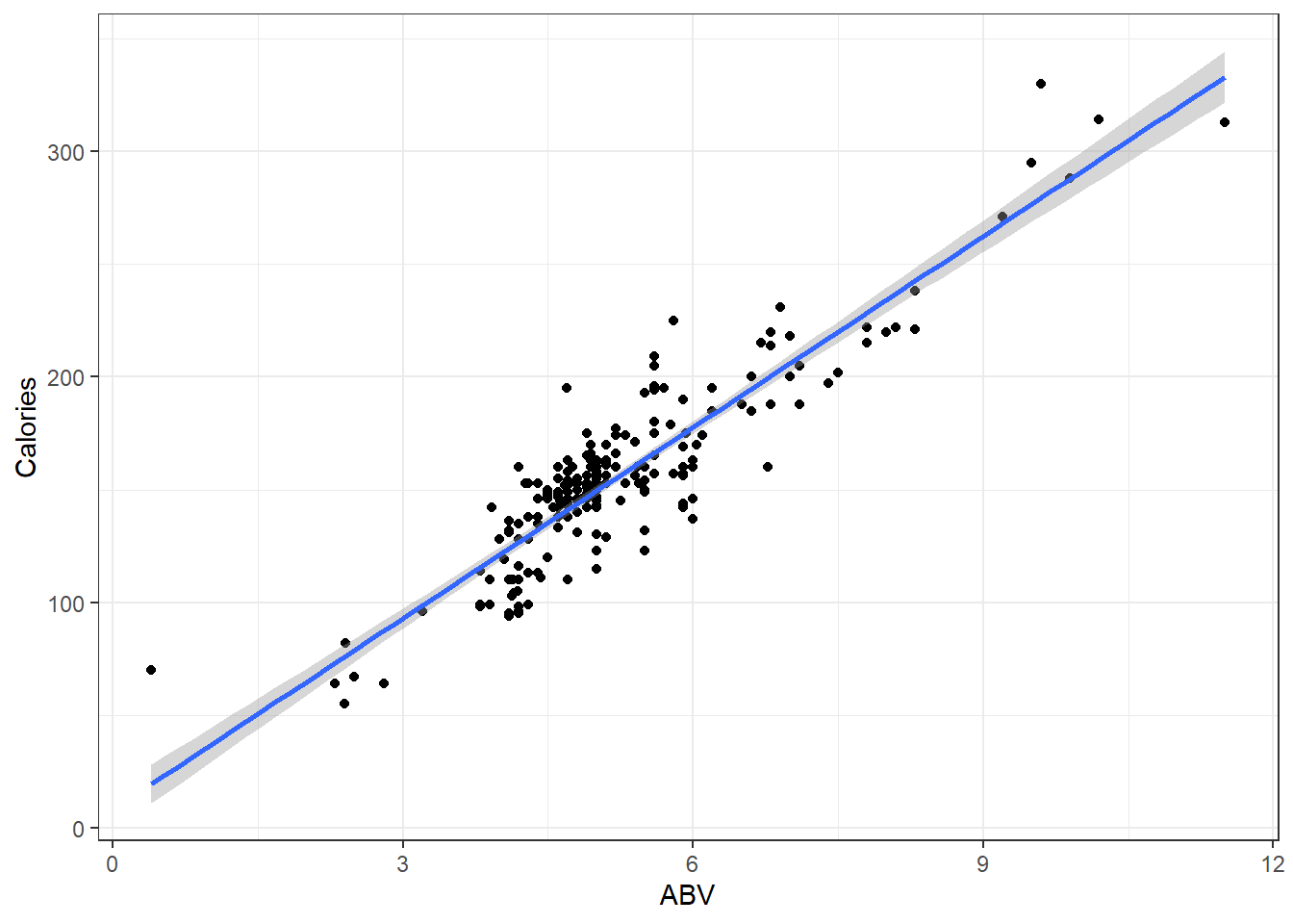
Additionally for the \(\epsilon \sim N(0, \sigma)\) term in the theoretical model,
Residual standard error: 17.48in our output tells us\(\hat \sigma = 17.48\) which means that at a given point on the line, we should expect the calorie content of individuals beers to fall above or below the line by about 17.48 calories.
4.2.4 Interpreting Coefficients
So we’ve got the slope estimate \(\hat \beta_i\) and we’ve got the intercept estimate \(\hat \beta_0\).
In general:
The slope tells us how much we expect the mean of our \(y\) variable to change when the \(x\) variable increases by 1 unit.
The intercept tells us what we would expect the mean value of \(y\) to be when the \(x\) variable is at 0 units.
Sometimes the intercept does not make sense.
- This is usually because \(x = 0\) is not within the range of our data.
- Or impossible.
- Or near the \(x=0\) range, the relationship between
For our data:
- The intercept of \(8.2464\) indicates that the model predicts that the mean calorie content of “beers” with 0% ABV is 8.2464 calories.
- There are some beers that are advertised as “non-alcoholic”.
- They have “negligble” amounts of alcohol but it is non-zero.
- Whether this is completely sensical or not depends on what you define as a beer.
- The slope of 28.2485 indicates that when we look at the mean calorie of beers, it should be 28.2485 calories higher of beers with a 1% higher ABV.
- This makes sense, i.e., alcohol has calories so more alcohol means more calories.
You always should look at your results and ask your self, “Does this make sense”?
- Usually the question of y-intercept making sense or not is not really a useful one.
- We need a y-intercept to have a line, and very often the data and what is reasonably observable does not include observations where \(x \approx 0\).
4.2.5 Prediction Using The Line
For our beers data, for beers with 5% ABV, we would expect an average calorie content of
\[\hat \mu_{y|x} = 8.2364 + 28.2485\cdot 5 \]
= 149.4789
Great, but what if you tell me you make beer at home and measure the ABV to be 5%.
- How many calories are in that specific Beer?
- We could say approximately 150 calories but that let’s not forget that we have an estimated error standard deviation of \(\hat \sigma = 17.48\) so it might be better to say the calorie content is some where in the 131.9989 to 166.9589 range (if we’re using a bunch of decimal places.)
- Honestly when doing casual intreptations it might be better to say \(150 \pm 20\) because its all about imprecision anyway.
4.2.6 Predict Function in R
Use the predict() function to get estimates for the mean which can be point estimates/predictions.
- The point of a regression model is estimate some sort model, and the method for doing so is called
predict. It works like so:
predict(lmModel, newdata)- Here
lmModelis an already estimated model, andnewdatais a dataset (referred to as data frame in R) containing the new cases, real or imaginary, for which we want to make predictions.
# Create a dataset for predicting average calories in beers with ABVs of 1%,
# 2%, 3%, ..., 10% R can create this vector easily with the `:` operator.
# `A:B` creates a vector that starts at A and goes up by 1 until it reaches
# (but does not exceed) B 1:10 represents the vector c(1, 2, 3, 4, 5, 6, 7, 8,
# 9, 10)

predictionData = data.frame(ABV = 1:10)


predict(beers.lm, newdata = predictionData)
1 2 3 4 5 6 7 8
36.49494 64.74349 92.99203 121.24058 149.48913 177.73768 205.98623 234.23478
9 10
262.48333 290.73188 - If you do not correctly specify the correct vector name in your
newdataargument, thenpredictwill simply give you the fitted \(\hat y\) values for each point in your data.
4.3 Statistcal Inference in Linear Regression
ggplot(beer, aes(x = ABV, y = Calories)) + geom_point() + geom_smooth(method = "lm",
    se = TRUE)
There’s bands around that line.
- This represents the fact that we don’t know the true regression line and are trying to account for how imprecise our estimate is.
- It displays a continuum for plausible values of the true line \(\hat \mu_{y|x}\) based on our sample data.
4.3.1 Example
Let’s look at what happens when the true model is \(Y = 300 - 5x + \epsilon\) when \(\epsilon \sim N(0, 20)\) and we take a sample of 50 individuals.
- The sample observations will be plotted in blue.
- The estimated regression line from those observations will be red.
- The true line will be in black.
n = 50

set.seed(11)

# Need x values
dat <- data.frame(x = rnorm(n, 33, 5))  #n, mu, sigma

# need a value for coefficients.
B <- c(300, -5)  # don't forget the y-intercept.

# Deterministic portion
dat$mu_y <- B[1] + B[2] * dat$x

# Introducing error
dat$err <- rnorm(n, 0, 20)

dat$y <- dat$mu_y + dat$err

ggplot(dat, aes(x = x, y = y)) + geom_point(data = dat, mapping = aes(x = x, y = y),
    col = "blue") + geom_smooth(method = "lm", col = "red") + geom_abline(intercept = B[1],
    slope = B[2], col = "black") + theme_bw()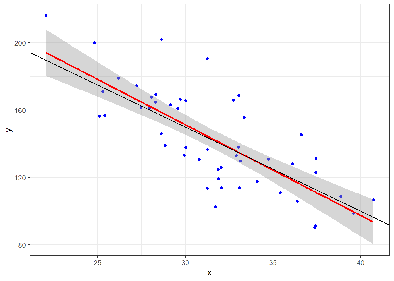
Given that we have sample data, we can’t expect our line to be the true line.
This is because there is variability associated with our slope estimate and variability associated with our intercept estimate.
4.3.2 Tests for the Line Coefficients
The \(\hat \beta\)’s are referred to as coefficients.
When you see the output for the summary of our lm, draw your attention to this part of the output.
    Coefficients:
            Estimate Std. Error t value Pr(>|t|)
(Intercept)   8.2464     4.7262   1.745   0.0824 .
ABV          28.2485     0.8857  31.893   <2e-16 ***
We are seeing various pieces of information. From left to right:
- We point estimates for the \(\hat beta\)’s.
- We are given standard errors for those estimates.
- We are given test statistics foir some hypothesis test (what is it)?
- We are given the p-value for that test.
The hypothesis test is this:
\[H_0: \beta_i = 0\] \[H_1: \beta_i \ne 0\]
The test statistic is:
\[t = \frac{\hat \beta_i}{SE_{\hat \beta_i}}\]
We simple divide our coefficient estimate by its standard error.
The test statistic is assumed to be from a \(t\) distribution with degrees of freedom \(df = n -2\).
For the y-intercept, we get a p-value of 0.0824:
- Our conclusion would be that there is moderate evidence that there is a true y-intercept in the model.
- Inference on the y-intercept is considered not important usually.
For the slope the p-value is approximately 0:
- Conclusion: There is extremely strong evidence of a linear component that relates ABV with calories.
- This is usually what we are concerned with.
4.3.3 Confidence Intervals
We can likewise get confidence intervals for the coefficients. They take the general form:
\[\hat \beta_i \pm t_{\alpha/2, \space n-2} \cdot SE_{\hat \beta_i}\]
Again the \(t_{\alpha/2}\) quantile depends on the value for \(\alpha\) of the desired nominal confidence level \(1 - \alpha\).
To get the confidence intervals we use the confint() function.
confint(beers.lm, level = 0.99) 0.5 % 99.5 %
(Intercept) -4.031982 20.52476
ABV 25.947491 30.54961Our interval indicates statistically plausible (which means disregarding context) levels for a y-intercept of the true line is between -4.03 and 20.52 with 99% confidence.
And plausible values for the increase in calories when beers have 1% higher ABV is between 25.95 and 30.55 with 99% confidence.
Do these CIs indicate any compatibility with the line for the theoretical line that computes (exactly) the amount of calories in a can of water with percentage of pure ethanol by volume?
\[f(x) = 19.05x\]