# Here are the libraries I used
library(tidyverse) # standard
# need for a couple things to make knitted document to look nice
library(knitr)
# need to read in data
library(readr)
# allows for stat_cor in ggplots
library(ggpubr)
# Needed for autoplot to work on lm()
library(ggfortify)
# allows me to organize the graphs in a grid
library(gridExtra)
 # need for some regression stuff like vif
library(car)
library(GGally)10 Outliers and Influential Observations
Here are some code chunks that setup this chapter.
# This changes the default theme of ggplot
old.theme <- theme_get()
theme_set(theme_bw())
10.1 Explainable statistical learning in public health for policy development: the case of real-world suicide data
We will work with data made available from this paper:
https://bmcmedresmethodol.biomedcentral.com/articles/10.1186/s12874-019-0796-7
If you want to go really in-depth of how you deal with data, this article goes into a lot of detail.
pheRed <- read_csv(here::here("datasets",
                              "phe_reduced.csv"))
10.1.1 Variables. A LOT!
colnames(pheRed) [1] "children_youth_justice" "adult_carers_isolated_all_ages"
[3] "alcohol_admissions_p" "children_leaving_care"
[5] "depression" "domestic_abuse"
[7] "self_harm_persons" "opiates"
[9] "marital_breakup" "alone"
[11] "self_reported_well_being" "social_care_mh"
[13] "homeless" "alcohol_rx"
[15] "drug_rx_opiate" "suicide_rate" 10.2 We have a model!
Using stepwise regression, we (supposedly) got a “good” model for “predicting” suicide rates:
fullModel <- lm(suicide_rate ~ ., pheRed)

model <- step(fullModel, trace = 0)

summary(model)
Call:
lm(formula = suicide_rate ~ children_leaving_care + self_harm_persons +
    opiates + marital_breakup + social_care_mh + homeless, data = pheRed)

Residuals:
    Min      1Q  Median      3Q     Max
-4.2494 -1.1217 -0.1575  0.9558  4.1356

Coefficients:
                        Estimate Std. Error t value Pr(>|t|)
(Intercept)            4.8392785  1.4371175   3.367 0.000977 ***
children_leaving_care  0.0423124  0.0197194   2.146 0.033595 *
self_harm_persons      0.0056140  0.0022875   2.454 0.015329 *
opiates                0.1055031  0.0507785   2.078 0.039537 *
marital_breakup        0.1878726  0.1344548   1.397 0.164505
social_care_mh         0.0008995  0.0004784   1.880 0.062108 .
homeless              -0.2066931  0.0749597  -2.757 0.006593 **
---
Signif. codes:  0 '***' 0.001 '**' 0.01 '*' 0.05 '.' 0.1 ' ' 1

Residual standard error: 1.69 on 142 degrees of freedom
Multiple R-squared:    0.4, Adjusted R-squared:  0.3746
F-statistic: 15.78 on 6 and 142 DF, p-value: 7.784e-14autoplot(model)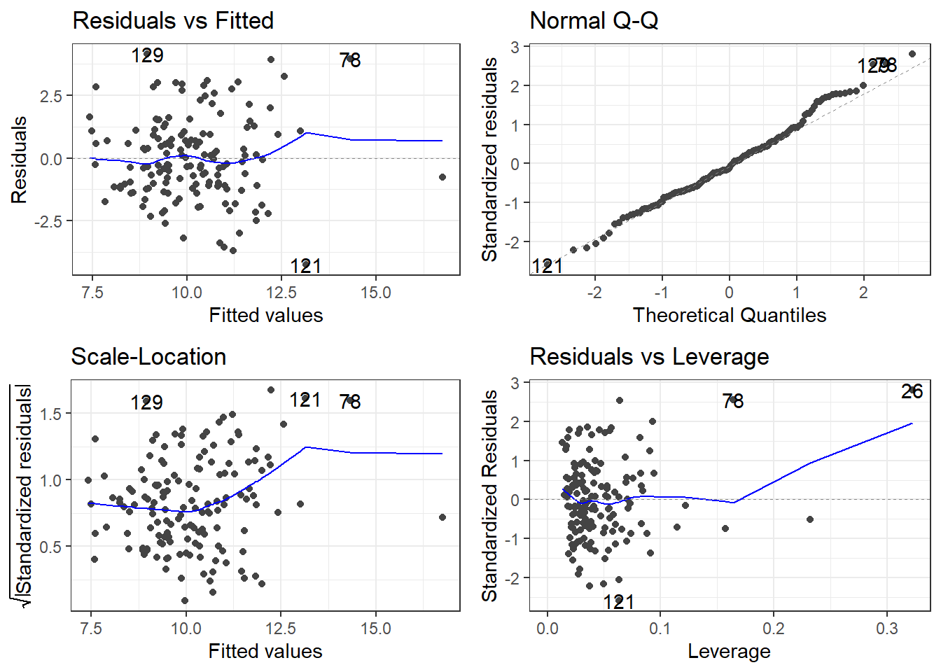
Is this a good model? Maybe, but there appear to be outliers.
Now we are going to learn more about that bottom left plot.
10.3 Leverage and Influence
We have several observations in our dataset which are composed an observed value of \(y_i\) and the corresponding predictor variables \(x_{1i}, x_{2i}, \dots, x_{p_i}\).
We make a prediction
\[\widehat y_i = \widehat \beta_0 + \widehat \beta_1 x_{1i} + \widehat \beta_{2} x_{2i} + ... + \widehat \beta_{p} x_{pi}\]
Leverage is how much potential influence an observation has on a regression line.
Leverage for the \(i^{th}\) observation in a dataset is denoted by \(h_i\).
Leverage is a measure of how far \(x_{1i}, x_{2i}, \dots, x_{p_i}\) deviate from the rest of the predictor variable observations.
Influence is a measure of how much of an effect the \(i^{th}\) observation has on the regression line/surface.
10.3.1 Low/High leverage versus Low/High Influence
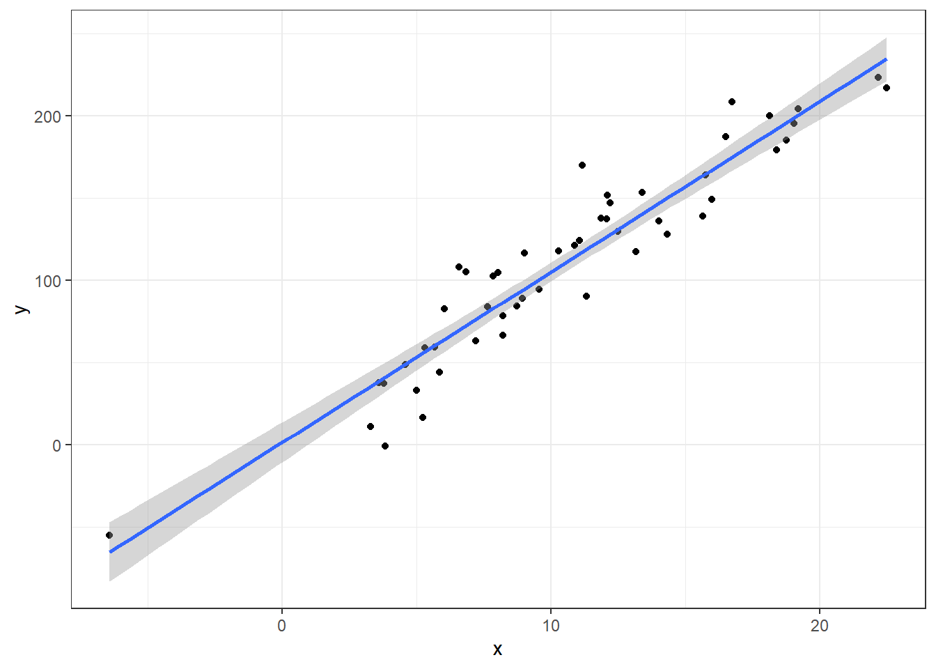
For simplicities sake, we’ll look at this with just simple linear regression model.
Here’s a regression model with perfectly well behaved
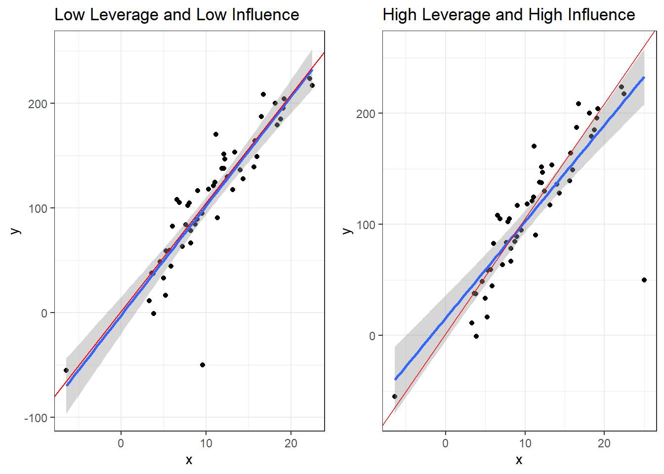
Now here are two plots. They each have an outlier. In red is the regression line that results from the outlier being removed.
The left plot has an outlier that is close to the mean of \(x\), and therefore has low leverage. Since the lines are close, this the outlier is low influence.
The one one the right shows an outlier with high distance from the center of \(x\) equating to high leverage. The discrepancy between the lines with and without the outlier indicates high influence.
Coefficients for model with no outliers:
coeff.summary(lm(y~x, data))| term | estimate | std.error | statistic | p.value |
|---|---|---|---|---|
| (Intercept) | 1.557531 | 6.0350674 | 0.2580802 | 0.7974484 |
| x | 10.371824 | 0.5021057 | 20.6566558 | 0.0000000 |
Coefficients for the the model with a high leverage but low influence outlier.
coeff.summary(lm(y~x, dat1))| term | estimate | std.error | statistic | p.value |
|---|---|---|---|---|
| (Intercept) | -2.437782 | 8.7784764 | -0.2776999 | 0.7824111 |
| x | 10.469077 | 0.7329583 | 14.2833181 | 0.0000000 |
Coefficients for the the model with a high leverage but high influence outlier.
coeff.summary(lm(y~x, dat2))| term | estimate | std.error | statistic | p.value |
|---|---|---|---|---|
| (Intercept) | 15.698247 | 10.1014749 | 1.554055 | 0.1266071 |
| x | 8.697335 | 0.8142884 | 10.680903 | 0.0000000 |
10.4 Finding High Influence Points
There are three main methods for determining high influence points:
- DFFITS: Determines effect of observation \(i\) on its estimate \(\widehat{y}_i\).
- Cook’s Distance (Cook’s D): Determines effect of an observation on the overall regression surface.
- Cook’s D and DFFITS are nearly identical accept for some slight tweaks. They have different cutoffs for “troublesome” values but tend to agree.
- DFBETAS: Determines effect of an observation on the each individual predictor coefficient.
- Influence is determined by an observation being an outlier with respect to a predictor variable.
- Some outliers only are outliers in terms of a single predictor variable.
10.4.1 DFFITS
- \(\widehat y_i\) is the predicted value of observation \(i\) in the data.
- \(\widehat y_{i(i)}\) is the predicted value of observation \(i\) in the data when the regression line is computed without observation \(i\).
- The notation kind of sucks, IMO, but it’s difficult to communicate the information in such a compact form. Just repeat the definitions in your head 10 times.
- \(h_i\) is the leverage of observation \(i\).
- \(MSE_{(i)}\) is the MSE of the regression model without observation \(i\).
If \(\widehat{y_i}\) and \(\widehat{y_{i(i)}}\) differ by a “substantial” relative to the leverage, then the outlier may be considered problematic
\[DFFITS_i = \frac{\widehat y_i - \widehat y_{i(i)}}{\sqrt{MSE_{(i)}\cdot h_i}}\]
There are a few different ways of determining if an observation has a “large” DFFITS value.
- For small to medium datasets, a \(DFFITS\) exceeding 1 (or -1) is problematic.
- For large datasets a \(DFFITS\) exceeding \(2\sqrt{p/n}\). Personally, I’d recommend \(3\sqrt{p/n}\) since DFFITS values are related to the \(t\) distribution.
- Recall \(p\) is the number of predictors.
- I’d say consider “large” to be 200 to 300 or more.
- This stuff is from way back when getting “large” amounts of data was quite a bit harder/expensive.
- Defining “large” is such an ephemeral thing given this age of “big” data.
10.4.2 Cook’s Distance (D)
For obersvation \(i\), Cook’s Distance \(D_i\) is:
\[D_i = \frac{\sum_{i=1}^n (\widehat y_i - \widehat y_{i(i)})}{p\cdot MSE}\] * Investigate observations with \(D_i > 0.5\), though some suggest \(D_i > 1\). * Cutoffs are a mess honestly, you shold look for \(D_i\) values that stick out and investigate.
10.4.3 DFBETAS
\(DFBETA_{k(i)}\) is a measure of how much observation \(i\) affects the estimated coefficient \(\widehat{\beta}_k\)
- \(\widehat{\beta}_k\) is the estimated coefficient using the whole dataset.
- \(\widehat{\beta}_{k(i)}\) estimated coefficient when observation \(i\) is removed from the data.
- \(k = 0,1,2,\dots p\)
- \(MSE_{(i)}\) is the MSE of the regression model without observation \(i\).
\[DFBETA_{k(i)} = \frac{\widehat{\beta}_k - \widehat{\beta}_{k(i)}}{\sqrt{MSE_{(i)} c_{kk}}}\] * A simple cutoff for \(DFBETA_{k(i)} > 1\) indicates observation \(i\) has a large effect on coefficient \(k\). * In this situation, you should care what happens to the \(y\)-intercept \(\widehat{\beta}_0\)
- $c_{kk} is a value computed using matrix theory. We aren’t a theory course so just trust me, it’s a number that should be there. It will be caclulated for you.
10.4.4 Custom Functions: Influential Observations calculator
In R, you do not need to install packages if you know how to program your own function.
You can create a function that does what you want. Here is a function that calculates all of the influence measures for all the observations in your dataset.
Just run the code-chunk and now you can use the function.
influence.measures <- function (model){
    is.influential <- function(infmat, n) {
        k <- ncol(infmat) - 2
        if (n <= k)
            stop("too few cases, n < k")
        absmat <- abs(infmat)
        result <- cbind(absmat[, 1L:k] > 1, absmat[, k + 1] >
            1, infmat[, k + 2]> 0.5)
        dimnames(result) <- dimnames(infmat)
        result
    }
    infl <- influence(model)
    p <- model$rank
    e <- weighted.residuals(model)
    s <- sqrt(sum(e^2, na.rm = TRUE)/df.residual(model))
    mqr <- stats:::qr.lm(model)
    xxi <- chol2inv(mqr$qr, mqr$rank)
    si <- infl$sigma
    h <- infl$hat
    dfbetas <- infl$coefficients/outer(infl$sigma,
                                       sqrt(diag(xxi)))
    vn <- variable.names(model)
    vn[vn == "(Intercept)"] <- "1_"
    colnames(dfbetas) <- paste("dfb", vn, sep = ".")
    dffits <- e * sqrt(h)/(si * (1 - h))
    if (any(ii <- is.infinite(dffits)))
        dffits[ii] <- NaN
    cooks.d <- (if (inherits(model, "glm"))
        (infl$pear.res/(1 - h))^2 * h/(summary(model)$dispersion *
            p)
    else ((e/(s * (1 - h)))^2 * h)/p)
    infmat <- cbind(dfbetas, dffit = dffits,
        cook.d = cooks.d)
    infmat[is.infinite(infmat)] <- NaN
    is.inf <- is.influential(infmat, sum(h > 0))
    infmat %>%
      as.data.frame() %>%
      mutate(influential = apply(is.inf, 1, any))
}
10.4.5 Influence Measures on PHE data
TRUE or FALSE is indicated in the right most column influential for observations that are declared “influential” accoding to the cutoffs discussed.
check <- influence.measures(model)

### This filters out any observations that are marked as "influential"

filter(check, influential)
dfb.1_ dfb.children_leaving_care dfb.self_harm_persons dfb.opiates
26 -0.2156744 0.19024198 0.13998317 -0.5959013
78 0.1388500 0.08110425 0.07286781 0.7102005
dfb.marital_breakup dfb.social_care_mh dfb.homeless dffit cook.d
26 0.06112809 1.908796 0.05305668 1.987504 0.5367057
78 -0.39154530 0.405517 -0.21624790 1.151952 0.1821697
influential
26 TRUE
78 TRUE10.4.6 Plotting the Residuals, Cook’s Distance and Leverage
- The
autoplotfunction has awhichargument. - It can create a total of 6 plots, each one having to do with residuals and influence measures.
autoplot(model, which = c(1, 2, 3, 4, 5, 6))will plot all 6.- Plot 1 is Residuals vs Fitted
- Plot 2 is the Normal Q-Q plot
- Plot 3 is the scale-location plot,
- Plot 4 is a plot of Cook’s distance for each observation.
- Plot 5 is Residuals vs Leverage
- Plot 6 is Cook’s Distance vs Leverage
- Remove any numbers for plots you don’t want.
My personal preference would be 1, 2, 4, 5.
autoplot(model, which = c(1, 2, 4, 5))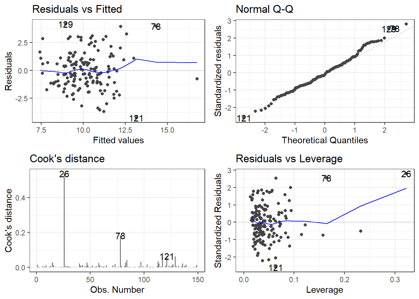
The top left is the raw residuals, this is where we assess the bias and constant variance.
The bottom right, are residuals calculated based on leverage.
- If the Standardized/Studentized Residual gets close to a value of 3, it may be problematic.
Studentized Residuals (Sometimes called Standardized Residuals):
\[t_i = \frac{e_i}{\sqrt{MSE_{(i)}(1-h_i)}}\]
It is EXTREMELY frustrating the language used.
Sometimes Standardized Residuals are:
\[t_i = \frac{e_i}{\sqrt{MSE}}\]
Which doesn’t account for leverage.
autoplot(model, which = c(3,5))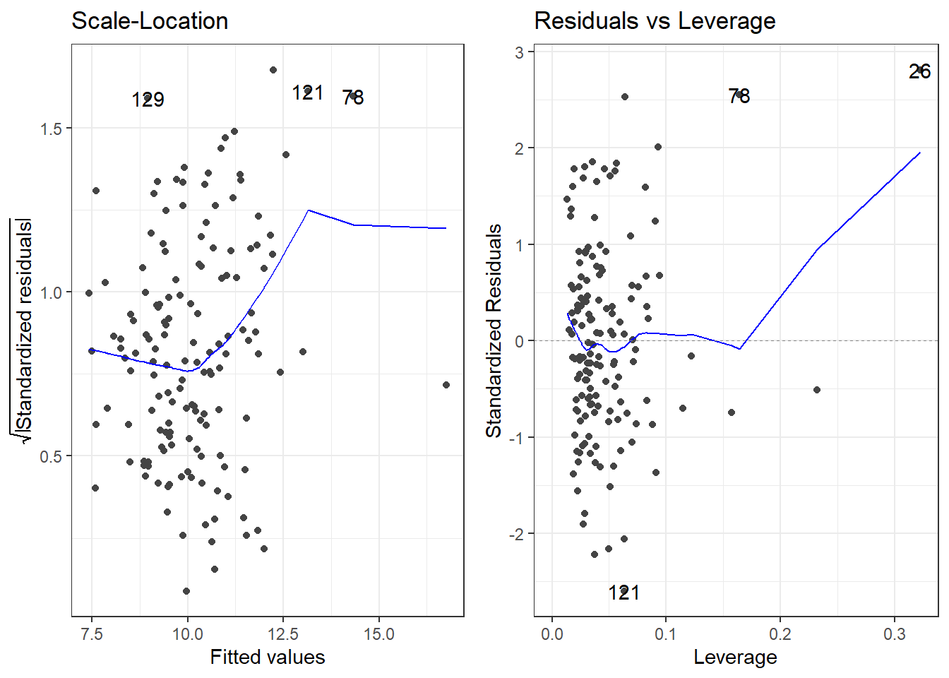
If both plots used the same definition of standard residuals, the marked observations which are the three most extreme residuals should be the observations.
:eyeroll:
10.5 You found some values that are high influence outliers, now what?
If there are only a couple per 200 or so, you can probably just delete them and not worry about it. If you have several, then there might be a bigger issue.
Ideally, you have more intimate knowledge of the data and would identify why outliers are not representative of the general population you are trying to model. If so, deletion probably is just fine.
Anyway, let’s pretend that that we can delete the two observations.
Let’s start with the worst one, 26.
10.5.1 Removing 26
pheOut1 <- pheRed[-26, ]

modelOut1 <- lm(suicide_rate ~ children_leaving_care + self_harm_persons +
    opiates + marital_breakup + social_care_mh + homeless, pheOut1)

summary(model)
Call:
lm(formula = suicide_rate ~ children_leaving_care + self_harm_persons +
    opiates + marital_breakup + social_care_mh + homeless, data = pheRed)

Residuals:
    Min      1Q  Median      3Q     Max
-4.2494 -1.1217 -0.1575  0.9558  4.1356

Coefficients:
                        Estimate Std. Error t value Pr(>|t|)
(Intercept)            4.8392785  1.4371175   3.367 0.000977 ***
children_leaving_care  0.0423124  0.0197194   2.146 0.033595 *
self_harm_persons      0.0056140  0.0022875   2.454 0.015329 *
opiates                0.1055031  0.0507785   2.078 0.039537 *
marital_breakup        0.1878726  0.1344548   1.397 0.164505
social_care_mh         0.0008995  0.0004784   1.880 0.062108 .
homeless              -0.2066931  0.0749597  -2.757 0.006593 **
---
Signif. codes:  0 '***' 0.001 '**' 0.01 '*' 0.05 '.' 0.1 ' ' 1

Residual standard error: 1.69 on 142 degrees of freedom
Multiple R-squared:    0.4, Adjusted R-squared:  0.3746
F-statistic: 15.78 on 6 and 142 DF, p-value: 7.784e-14summary(modelOut1)
Call:
lm(formula = suicide_rate ~ children_leaving_care + self_harm_persons +
    opiates + marital_breakup + social_care_mh + homeless, data = pheOut1)

Residuals:
    Min      1Q  Median      3Q     Max
-3.8140 -1.0888 -0.0478  0.8991  4.2533

Coefficients:
                        Estimate Std. Error t value Pr(>|t|)
(Intercept)            5.142e+00  1.405e+00   3.658 0.000358 ***
children_leaving_care  3.865e-02  1.927e-02   2.006 0.046811 *
self_harm_persons      5.302e-03  2.233e-03   2.374 0.018957 *
opiates                1.350e-01  5.057e-02   2.670 0.008479 **
marital_breakup        1.799e-01  1.312e-01   1.371 0.172448
social_care_mh         9.008e-06  5.596e-04   0.016 0.987180
homeless              -2.106e-01  7.312e-02  -2.880 0.004598 **
---
Signif. codes:  0 '***' 0.001 '**' 0.01 '*' 0.05 '.' 0.1 ' ' 1

Residual standard error: 1.648 on 141 degrees of freedom
Multiple R-squared:  0.4011,    Adjusted R-squared:  0.3756
F-statistic: 15.74 on 6 and 141 DF,  p-value: 8.76e-14
The biggest change is in the social_care_mh variable. It seems almost complete useless now.
autoplot(modelOut1, which = c(1, 2, 4, 5))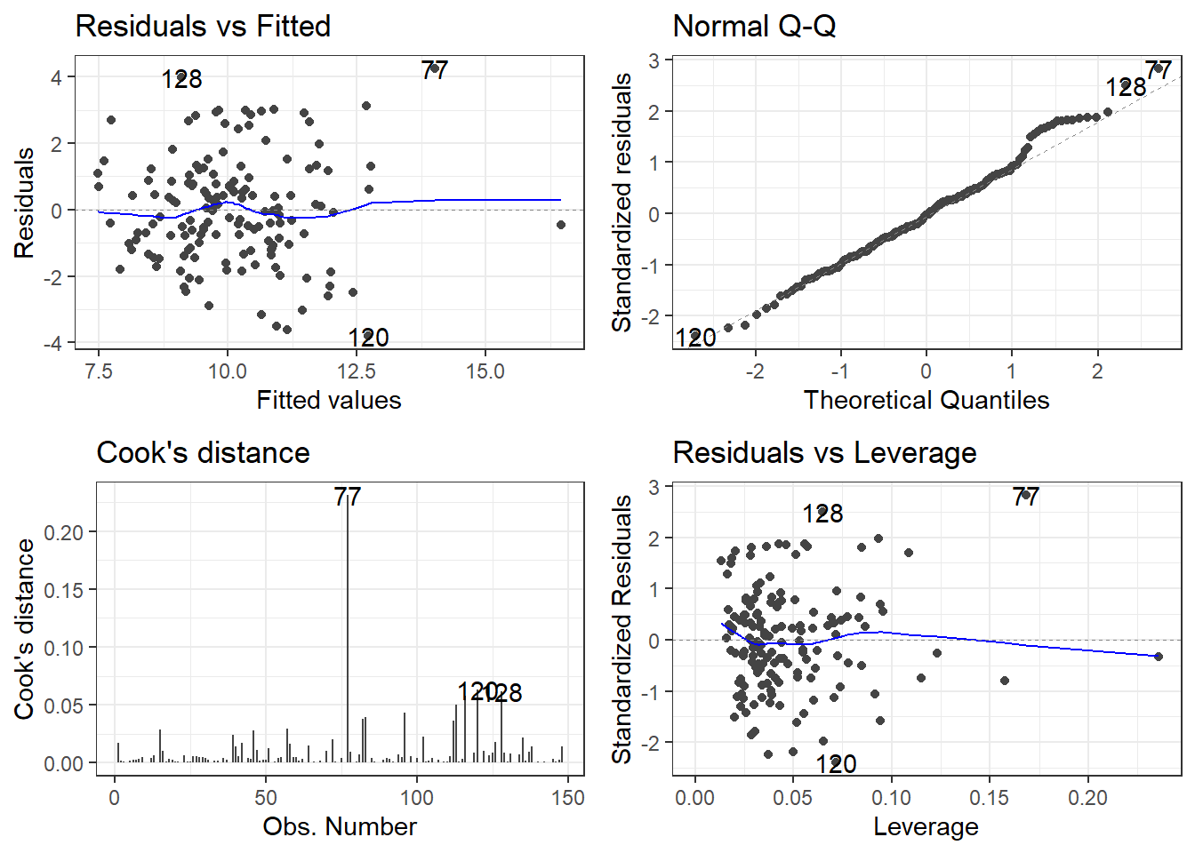
10.5.2 Does stepwise
What if we did stepwise regression?
fullModelOut1 <- lm(suicide_rate ~ ., pheOut1)
stepModelOut1 <- step(fullModelOut1,
                      direction = "both", trace = 0)

summary(stepModelOut1)
Call:
lm(formula = suicide_rate ~ children_leaving_care + self_harm_persons +
    opiates + homeless, data = pheOut1)

Residuals:
    Min      1Q  Median      3Q     Max
-3.8571 -1.0684  0.0412  1.0111  4.1770

Coefficients:
                       Estimate Std. Error t value Pr(>|t|)
(Intercept)            6.936358   0.526026  13.186  < 2e-16 ***
children_leaving_care  0.044349   0.018584   2.386  0.01832 *
self_harm_persons      0.006252   0.002120   2.948  0.00373 **
opiates                0.133822   0.048731   2.746  0.00681 **
homeless              -0.222190   0.072526  -3.064  0.00261 **
---
Signif. codes:  0 '***' 0.001 '**' 0.01 '*' 0.05 '.' 0.1 ' ' 1

Residual standard error: 1.647 on 143 degrees of freedom
Multiple R-squared:  0.393, Adjusted R-squared:  0.376
F-statistic: 23.15 on 4 and 143 DF,  p-value: 9.143e-15
Now stepwise regression says the best model (according to AIC) appears to now only have four variables with marital_breakup and social_care_mh now out of the model.
autoplot(stepModelOut1, which = c(1, 2, 4, 5))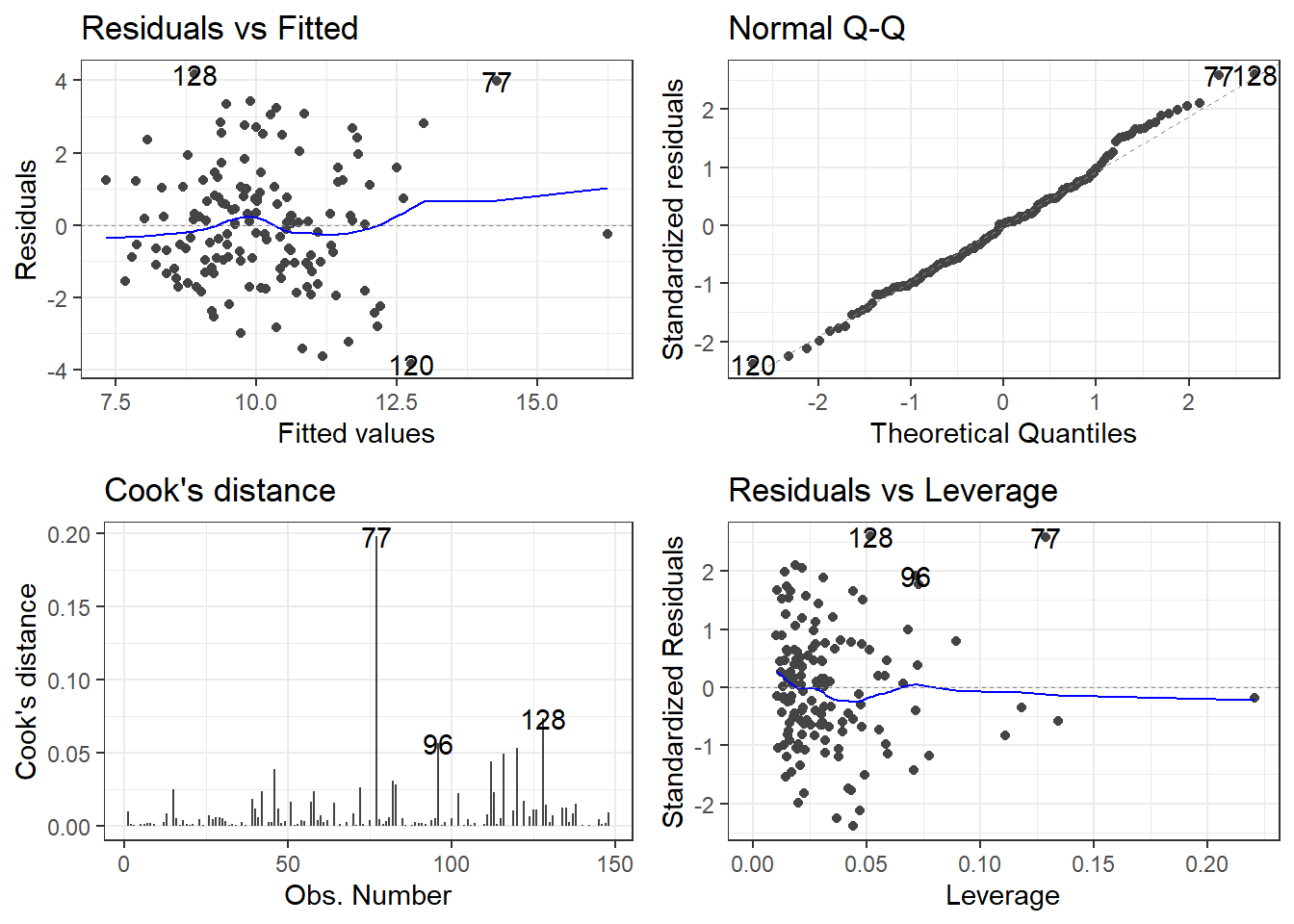
10.5.3 Removing the other outlier
The other outlier in the original data was 78, which is now 77 in the data with the first outlier removed.
pheOut2 <- pheRed[-c(26, 78), ]
modelOut2 <- lm(suicide_rate ~ children_leaving_care + self_harm_persons +
    opiates + marital_breakup + social_care_mh + homeless, pheOut2)

summary(modelOut2)
Call:
lm(formula = suicide_rate ~ children_leaving_care + self_harm_persons +
    opiates + marital_breakup + social_care_mh + homeless, data = pheOut2)

Residuals:
    Min      1Q  Median      3Q     Max
-3.6411 -1.1723 -0.0252  0.9400  3.7675

Coefficients:
                        Estimate Std. Error t value Pr(>|t|)
(Intercept)            4.9507489  1.3713937   3.610 0.000426 ***
children_leaving_care  0.0366938  0.0187964   1.952 0.052914 .
self_harm_persons      0.0051023  0.0021779   2.343 0.020552 *
opiates                0.0987500  0.0508446   1.942 0.054121 .
marital_breakup        0.2352779  0.1292469   1.820 0.070838 .
social_care_mh        -0.0002604  0.0005533  -0.471 0.638623
homeless              -0.1936071  0.0715014  -2.708 0.007619 **
---
Signif. codes:  0 '***' 0.001 '**' 0.01 '*' 0.05 '.' 0.1 ' ' 1

Residual standard error: 1.606 on 140 degrees of freedom
Multiple R-squared:  0.3686,    Adjusted R-squared:  0.3416
F-statistic: 13.62 on 6 and 140 DF,  p-value: 3.809e-12
What does stepwise regression say now?
fullModelOut2 <- lm(suicide_rate ~ ., pheOut2)
stepModelOut2 <- step(fullModelOut2, direction = "both", trace = 0)

summary(stepModelOut2)
Call:
lm(formula = suicide_rate ~ children_leaving_care + self_harm_persons +
    opiates + marital_breakup + homeless, data = pheOut2)

Residuals:
    Min      1Q  Median      3Q     Max
-3.6265 -1.1113 -0.0436  0.9571  3.8287

Coefficients:
                       Estimate Std. Error t value Pr(>|t|)
(Intercept)            4.926482   1.366636   3.605 0.000432 ***
children_leaving_care  0.038065   0.018518   2.056 0.041667 *
self_harm_persons      0.005157   0.002169   2.378 0.018764 *
opiates                0.093673   0.049550   1.890 0.060745 .
marital_breakup        0.228541   0.128097   1.784 0.076553 .
homeless              -0.192514   0.071266  -2.701 0.007753 **
---
Signif. codes:  0 '***' 0.001 '**' 0.01 '*' 0.05 '.' 0.1 ' ' 1

Residual standard error: 1.602 on 141 degrees of freedom
Multiple R-squared:  0.3676,    Adjusted R-squared:  0.3452
F-statistic:  16.4 on 5 and 141 DF,  p-value: 9.804e-13
And now marital_breakup breakup is back in?
autoplot(stepModelOut2)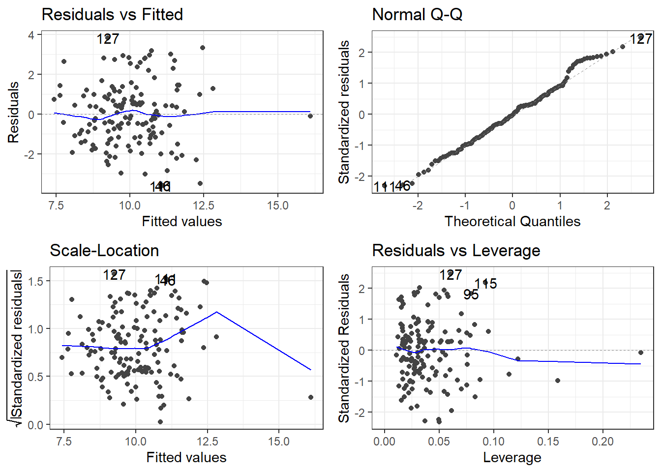
10.6 Which model to use
In short, there is no good answer.
- If you have absolutely no idea what’s going on and all you care about is prediction accuracy, the stepwise regression approach may (read: MAY) be okay.
- This is an acceptable approach within exams and assignments for this course, but should be scrutinized in real world modeling.
- If you know more about what’s going on and have specific experimental questions, then use the models proposed by those questions and look at how useful they are.
- That’s kind of what they did in the paper.
There is no correct way to go about this.
10.7 Our model building process
- Look at the full model. Coefficients, residuals, and all.
- Investigate for multicollinearity and find ways to remove variables that may be problematic.
- Look at the full model of the reduced data: coefficients, residuals, and all. You may need to apply a transformation to the \(y\) variable.
- If you think it’s a good fit and can justify using it, you’re done.
- Otherwise you need to start eliminating variables via knowledge of the data or specific experimental questions ideally. If you are purely aiming for a predictive approach, you may try stepwise regression. It is best to try all methods, but stepwise in both directions is acceptable in this class.
- Once you have found a reduced model, examine the residuals for outliers and violation assumptions. Remove outliers if you can justify it.
- If you don’t have outliers and your assumptions look good, you’re done.
- Check if your variables still remain relevant. You may have to remove or add variables that are now relevant. Use experimental questions or stepwise regression again…
- Check residuals and outliers again. Hopefully everything looks. Good.
Everytime you messed with something in the model, you need to go back through and check residuals, validity of transformations, etc.
I’ll throw you softballs in this class for the sake of your sanity.