14 Balanced (Uniform Sample Size) Two-Way ANOVA

Here are some code chunks that setup this chapter

# Here are the libraries I used
library(tidyverse) # standard
library(knitr) 
library(readr) 
library(ggpubr) # allows for stat_cor in ggplots
library(ggfortify) # Needed for autoplot to work on lm()
library(gridExtra) # allows me to organize the graphs in a grid
library(car) # need for some regression stuff like vif
library(GGally)
library(emmeans)

# This changes the default theme of ggplot
old.theme <- theme_get()
theme_set(theme_bw())

The idea of analysis of variance mainly stems from concepts of “experimental design” which is a separate course that should be taken should you be in a field that heavily focuses on, well… quantitative experiments that will be analyzed.

There is so much there that we can’t even touch on it in a meaningful way with the scope of this course.

Anyway, in an experiment we manipulate external variables and see their affect on the response variable.

\(y\) is our response variable
We can have various \(x\) variables that we are manipulating.
- In ANOVA context these are called factors.
- We can have more than one factor. (Technically as many as we want, but probably stop at 3!)
- Each factor has a set of levels, i.e. the specific values that are set
- A treatment is the specific combination of the levels of all the factors.
- Each individual treatment could be referred to as a cell.
Group A: A_1_,A_2_,A_3_
Group B: B_1_, B_2_
Group Combinations: A_1_B_1_,A_2_B_1_,A_3_B_1_,A_1_B_2_,A_2_B_2_,A_3_B_2_

14.1 Pseudo-Example

We are doing an ANOVA type experiment.

We have are subjects and we want to test the effectiveness of a drug and exercise regime on blood pressure.
The drug is factor A and there will be 3 dose levels: 0mg (control), 5mg, and 10mg
The exercise regime is factor B with 3 levels: none (control), light, heavy.
This would be referred to as a 3 by 3 (\(3\times3\)) ANOVA.
- In general we say \(A\times B\) where we put the number of levels for each factor.
- In this case there would be 9 total unique combinations of the two factors which means there would be 9 treatments

We can view it as a grid kind of pattern for the design of the experiement.

Regime\Dose	0mg	5mg	10mg
none	0 & none (control)	5 & none	10 & none
light	0 & light	5 & light	10 & light
heavy	0 & heavy	5 & heavy	10 & heavy

And there would be a random assignment of each treatment to a set of subjects.

14.1.1 Sample Sizes in Two-Way ANOVA

A basic analysis is possible if there is only one subject per treatment (cell).
- This is not an ideal scenario.
More than 1 subject per treatment is better.
An equal number of subjects for each treatment is “best”, which is called a balanced design
- This may not feasible many times when involving living individuals (humans or otherwise.
- Subject smay drop out of studies for various reasons.
- Levels of factors may have different difficulties for obtaining/producing.
- Variability of subject availability depending on treatments.
- Etc.
If there are not an equal number of individuals within each group, it is referred to as an unbalanced design.
This usually not a problem with a large enough sample size and when there isn’t heteroscedasticity (check your assumptions!)

We will cover Balanced Design.

Unbalanced Design requires much more care and you should consult someone with experience.

Should time allow, we will cover it. But it really is just a mess to wrap your head around.

14.2 Notation and jargon

There’s a lot here. The notation logic is fairly procedural (to a degree that it becomes confusing).

Factors and Treatments

We have factor A with levels \(i = 1,2, \dots, a\) and factor B with levels \(j = 1,2, \dots, b\).

\(A_i\) represents level \(i\) of factor \(A\).
\(B_j\) represents level \(j\) of factor \(B\).
\(A_iB_j\) represents the treatment combination of level \(i\) and level \(j\) of factors A and B respectively.
This is sometimes referred to as “treatment ij”.

Observations and Sample Means

An individual observation is denoted by \(y_{ijk}\). The subscripts indicate we are looking at observation \(k\) from treatment \(A_iB_j\)

There are \(n\) observations in each individual treatment treatment, \(k = 1,2, \dots, n\).
\(\overline y_{ij.}\) is the mean of the observations in treatment \(A_iB_j\). (\(\overline y_{ij.} =\frac{1}{n} \sum_{k=1}^{n}y_{ijk}\))
\(\overline y_{i..}\) is the mean of the observations in treatment \(A_i\) across all levels of factor B. (\(\overline y_{i..} = \frac{1}{bn}\sum_{j=1}^{b}\sum_{k=1}^{n}y_{ijk}\))
\(\overline y_{.j.}\) is the mean of the observations in treatment \(B_j\) across all levels of factor A. (\(\overline y_{.j.} = \frac{1}{an}\sum_{i=1}^{a}\sum_{k=1}^{n}y_{ijk}\))
\(\overline y_{...}\) is the mean of all observations. (\(\overline y_{...} = \frac{1}{abn}\sum_{i=1}^{a}\sum_{j=1}^{b}\sum_{k=1}^{n}y_{ijk}\))

14.3 Two way ANOVA Model

There is a means model:

\[y = \mu_{ij} + \epsilon\]

\(\mu_{ij}\) is the mean of treatment \(A_iB_j\).
Epsilon is the error term and it is assumed \(\epsilon \sim N(0, \sigma)\).
- The constant variability assumption is here.

Which in my opinion is not congruent with what we are trying to investigate in Two-Way ANOVA.

We are trying to understand the effect that both factors have on the the response variable.
There may be an interaction between the factors.
- This is when the effect the levels of factor A is not consistent across all levels of factor B, and vice versa.
- For example, the mean of the response variable may increase when going from treatment \(A_1B_1\) to \(A_2B_1\), but the response variable mean decreases when we look at \(A_1B_2\) to \(A_2B_2\).

With this all in mind, the effects model in two-way ANOVA is:

\[y = \mu + \alpha_i + \beta_j + \gamma_{ij} + \epsilon\]

\(\mu\) would be the mean of the response variable without the effects of the factors.
- This can usually be thought of as the mean of a control group.
\(\alpha_i\) can be thought of as the effect that level \(i\) of factor A has on the mean of \(y\).
Likewise, \(\beta_j\) is the effect that level \(j\) of factor B has on the mean of \(y\).
\(\gamma_{ij}\) is the interaction effect, which is the additional effect that the specific combination \(A_i\) and \(B_j\) has on the mean of \(y\).

14.3.1 Estimating model parameters (Means model)

If we are considering a means model there are a few things we can consider:

The overall mean of the data \(\mu_{..}\) which is estimated by \(\overline y_{...}\)
The overall mean of \(A_i\) (when averaged over factor B) \(\mu_{i.}\) which is estimated by \(\overline y_{i..}\)
The overall mean of \(B_j\) (when averaged over factor B) \(\mu_{.j}\) which is estimated by \(\overline y_{.j.}\)
The treatment mean of \(A_iB_j\) \(\mu_{ij}\) which is estimated by \(\overline y_{ij.}\)

14.3.2 Estimating model parameters (Effects model)

It might be more interesting to estimate how big the effect is of a given treatment or how large an interaction is.

I would argue that the only meaningfully done IF there is a control group in both factors.

Assume that \(A_1\) and \(B_1\) are the control levels.

Then \(\alpha_1\) and \(\beta_1\) should be (at least conceptually) \(0\).
There would be no interaction terms for any treatment \(A_1B_j\) or \(A_iB_j\)
\(\widehat \alpha_i = \overline y_{i..} - \overline y_{1..}\)
\(\widehat \beta_i = \overline y_{.j.} - \overline y_{.1.}\)
\(\widehat \gamma_{ij} = \overline y_{ij.} - \overline y_{i1.} - \overline y_{1j.} + \overline y_{ij.}\)

Estimating the interactions involves things we call contrasts and that is another can of worms.

14.4 Hypothesis Tests

There are three sets of hypotheses that can potentially be tested in ANOVA.

14.4.1 Main Effects Tests

We can test whether factor A has an effect.

\(H_0: \alpha_i = 0\) for all \(i\), i.e., factor A has no effect on the mean of \(y\).

Note that this would be the hypothesis if there were a control group.
Otherwise it would be more correct to say that all levels of factor A have an equivalent effect (\(\alpha_1 = \alpha_2 = \dots = \alpha_a\))

\(H_1:\) \(\alpha_i \neq 0\) for at least one \(i\). At least one level of factor A has an effect on the mean of \(y\).

Or without a control, at least one \(\alpha_i\) differs from the rest.

Likewise we can perform a separate test for whether factor \(B\) has an effect:

\(H_0: \beta_j = 0\) for all \(j\), i.e., factor B has no effect on the mean of \(y\).

Note that this would be the hypothesis if there were a control group.
Otherwise it would be more correct to say that all levels of factor B have an equivalent effect (\(\beta_1 = \beta_2 = \dots = \beta_b\))

\(H_1:\) \(\beta_j \neq 0\) for at least one \(j\). At least one level of factor B has an effect on the mean of \(y\).

Or without a control, at least one \(\beta_i\) differs from the rest.

14.4.2 Interaction Test

BEFORE Before you can rely on the tests for the main effects, you must first consider testing for whether there is any meaningful interaction.

\(H_0\): \(\gamma_{ij} = 0\) for all \(A_iB_j\) treatment combinations.

The idea of changing the hypothesis for whether there is a control or not is a bit more technical.
You could say the effects are all equivalent but then there really isn’t an interaction.
There are multiple valid hypotheses IMO. So stick with this one to avoid getting too technical.

\(H_1: \gamma_{ij} \neq 0\) for at least on \(A_iB_j\) treatment combination.

The reason that this test must be the first one to be considered is that if there is an interaction effect, it becomes mathematically impossible to effectively conclude the strength of an effect of an individual factor overall.

Interaction implies the effect of one factor changes depending on another factor so statements about individual factors are a moot point.

14.4.3 Sums of Squares, Mean Squares, and Test Statistics

We are going to ignore all the formula based stuff at this point, just consider the concepts.

We measure how meaningful a factor or interaction is via sums of squares, just as before.
\(SSA\) measures how meaningful is factor A within the data.
- The degrees of freedom is \(a - 1\).
\(SSB\) measures how meaningful is factor B within the data.
- The degrees of freedom is \(b - 1\)
\(SSAB\) measures how meaningful is the interaction within the data.
- The degrees of freedom is \((a-1)(b-1)\)
\(SSE\) is the measure of how much variability is left unexplained by the factors and interaction.
- The degrees of freedom is \(ab(n-1)\)

“Meaningful” translates to “the amount of variability in data the data that is explained by including the variable in the model”.

Just as before, to get test statistics we need to compute mean squares.

\(MSA = SSA/(a-1)\)
\(MSB = SSB/(b-1)\)
\(MSAB = SSAB/(a-1)(b-1)\)
\(MSE = SSE/(ab(n-1))\)

And then we get \(F\) test statistics.

\(F_A = MSA/MSE\) tests whether factor A has an effect, \(H_0: \alpha_i = 0\) for all \(i\).
\(F_B = MSB/MSE\) tests whether factor B has an effect, \(H_0: \beta_j = 0\) for all \(j\).
\(F_{AB} = MSAB/MSE\) tests whether there is an interaction effect, \(H_0\): \(\gamma_{ij} = 0\) for all \(i\) and \(j\).

14.4.4 And so there is a Two-Way ANOVA table (surprise)

Source	SS	df	MS	F	p
Factor A	\(SSA\)	\(a-1\)	\(MSA=SSA/(a-1)\)	\(F_A = MSA/MSE\)	\(p_A\)
Factor B	\(SSB\)	\(b-1\)	\(MSB=SSB/(b-1)\)	\(F_B = MSB/MSE\)	\(p_B\)
Interaction: A*B	\(SSAB\)	\((a-1)(b-1)\)	\(MSAB = SSAB/((a-1)(b-1))\)	\(F_{AB} = MSAB/MSE\)	\(p_{AB}\)
Error	\(SSE\)	\(ab(n-1)\)	\(MSE = SSE/(ab(n-1))\)

Reject \(H_0\) if \(p < \alpha\)
\(P_A \rightarrow H_0: \alpha_i = 0\)
\(P_A \rightarrow H_0: \beta_j = 0\)
\(P_{AB} \rightarrow H_0: \gamma_i = 0\)

14.5 Study: Compulsive Checking and Mood

This data is taken from the textbook resources of: Discovering Statistics Using R by Andy Field, Jeremy Miles, Zoë Field

which itself is using data from a journal article (one textbook author is a paper co-author):

The perseveration of checking thoughts and mood–as–input hypothesis by Davey et al. (2003), https://doi.org/10.1016/S0005-7916(03)00035-1.

The study investigated the relation between mood and when people will stop performing a task under different stopping rules. They were trying to explore the connection with Obsessive Compulsive Disorder.

There were 60 participants (it was one of those college student studies).
The mood of a participant was “induced” via music:
- 20 were assigned to have a “negative” mood induction.
- 20 were assigned to have a “positive” mood induction.
- 20 were assigned to have a “neutral” mood induction.
Participants were then asked to “to write down all the things they would wish to check for safety or security reasons in their home before they left for a 3-week holiday”.
Within each mood group:
- 10 participants were told to continue the task only if they felt like continuing.
- 10 participants were told to continue the task until they’ve listed as many as they can.

Data are available in compulsion.csv.

items: how many items a participant listed.
mood: which mood induction group the participant was in.
- Negative
- Positive
- Neutral
stopRule: what was the stopping rule
- Many : “As many as you can”
- Feel : “Feel like continuing”

ocd <- read_csv(here::here("datasets",'ocd.csv'))

Here is what a sample of the data look like

# A tibble: 10 × 3
   items mood     stopRule
   <dbl> <chr>    <chr>   
 1     9 Negative Feel    
 2     8 Neutral  Feel    
 3    13 Negative Many    
 4     3 Negative Feel    
 5    10 Positive Many    
 6     7 Negative Feel    
 7     7 Negative Many    
 8     7 Neutral  Feel    
 9    14 Positive Feel    
10     4 Positive Many

For videos related to the analysis of this data in R, I’ll go over some issues with the analyses performed. We are basically following along with what was done in the paper.

14.5.1 Examining the data

Always take a look at your data first.

We’ll look at boxplots, you can group by mood and color by stopping rule.

ggplot(ocd, aes(y = items, x = mood, color = stopRule)) +
  geom_boxplot()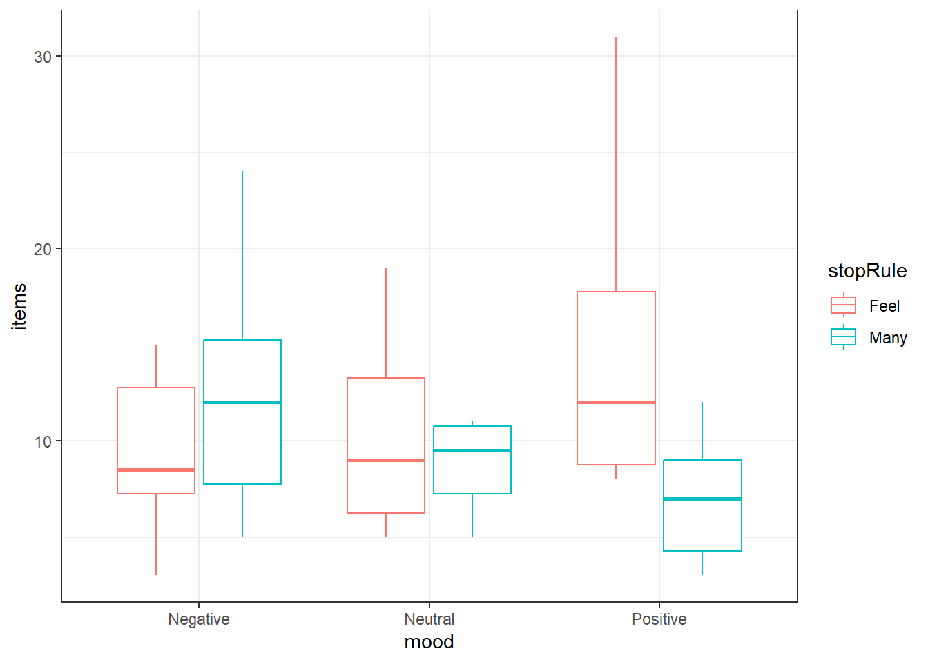

14.5.2 Performing two-way ANOVA

ANOVA is similar to before and we can add variables like in regression. There is a trick to adding in an interaction.

You specify the interaction of two variables by “multiplying” them with the : symbol in the formula, e.g., y ~ x + z + x:z

For two-way ANOVA, I highly recommend always using the Anova() function from the car package, not the Anova() function. The reason will be clarified

ocd.fit <- lm(items ~ mood + stopRule + mood:stopRule, 
              data = ocd)

car::Anova(ocd.fit)

Anova Table (Type II tests)

Response: items
               Sum Sq Df F value   Pr(>F)   
mood            34.13  2  0.6834 0.509222   
stopRule        52.27  1  2.0928 0.153771   
mood:stopRule  316.93  2  6.3452 0.003349 **
Residuals     1348.60 54                    
---
Signif. codes:  0 '***' 0.001 '**' 0.01 '*' 0.05 '.' 0.1 ' ' 1

Equivalently, you could “multiply” via the * symbol without listing the individual variables.

The * tells R to include all individual AND interaction terms when used in a formula, e.g., y ~ x*z

So equivalently we could do:

ocd.fit2 <- lm(items ~ mood*stopRule, data = ocd)
Anova(ocd.fit2)

Anova Table (Type II tests)

Response: items
               Sum Sq Df F value   Pr(>F)   
mood            34.13  2  0.6834 0.509222   
stopRule        52.27  1  2.0928 0.153771   
mood:stopRule  316.93  2  6.3452 0.003349 **
Residuals     1348.60 54                    
---
Signif. codes:  0 '***' 0.001 '**' 0.01 '*' 0.05 '.' 0.1 ' ' 1

And we get equivalent results.

14.6 Post-hoc Comparisons: Estimated Marginal Means

Depending how we want to view the data, the means we are interested in may change.

If we want to (and can) investigate the main effects, we look at what are referred to as the marginal means
- \(\overline y_{i..}\) is the marginal mean of level \(i\) of factor A. (Averaged across all levels of B)
- \(\overline y_{.j.}\) is the marginal mean of level \(j\) of factor B. (Averaged across all levels of A)
\(\overline y_{ij.}\)’s are known as the cell or treatment means. The mean of treatment \(A_iB_j\)

14.6.1 Using the `emmeans()` function to get marginal or cell means

The emmeans() function within the eponymous emmeans package.

We will stick with the simplest way.

The format is emmeans(model, specs, level = 0.95)
model is the lm or other type of model you create.
specs specifies what means you want and how you want to adjust them.
- The input is a formula style but without the response variable listed, i.e., ~ x and not y ~ x (unless you know some more “fun” stuff).
- ~ A will compute the marginal means for each level of factor A. This should only be used if an interaction term is not “significant”.
- ~ A | B will calculate the cell means for the levels of factor A conditioned upon what the level of factor B is.
- ~ A | B is a way of organizing the interaction means in a Two-Way model
- You can switch which variable. B | A.
- When you specify at condition variable using | you are getting only the a portion of the interaction means.
- ~ A*B will compute the cell/interaction means
level specifies the confidence level of resulting confidence interval
There is an adjust argument, it is tukey by default and lets just leave it like that.
- adjust with change automatically depending on the situation.

emmeans(ocd.fit, ~ mood, level = 0.99)

 mood     emmean   SE df lower.CL upper.CL
 Negative   10.9 1.12 54     7.92     13.9
 Neutral     9.3 1.12 54     6.32     12.3
 Positive   10.9 1.12 54     7.92     13.9

Results are averaged over the levels of: stopRule 
Confidence level used: 0.99

emmeans(ocd.fit, ~ mood | stopRule, level = 0.99)

stopRule = Feel:
 mood     emmean   SE df lower.CL upper.CL
 Negative    9.2 1.58 54     4.98     13.4
 Neutral     9.9 1.58 54     5.68     14.1
 Positive   14.8 1.58 54    10.58     19.0

stopRule = Many:
 mood     emmean   SE df lower.CL upper.CL
 Negative   12.6 1.58 54     8.38     16.8
 Neutral     8.7 1.58 54     4.48     12.9
 Positive    7.0 1.58 54     2.78     11.2

Confidence level used: 0.99

emmeans(ocd.fit, ~ mood:stopRule, level = 0.99)

 mood     stopRule emmean   SE df lower.CL upper.CL
 Negative Feel        9.2 1.58 54     4.98     13.4
 Neutral  Feel        9.9 1.58 54     5.68     14.1
 Positive Feel       14.8 1.58 54    10.58     19.0
 Negative Many       12.6 1.58 54     8.38     16.8
 Neutral  Many        8.7 1.58 54     4.48     12.9
 Positive Many        7.0 1.58 54     2.78     11.2

Confidence level used: 0.99

Note that it warns you that an interaction is present and therefore you should not look at single factor means. (How convenient.)

14.6.2 Getting pairwise comparisons

To get pairwise comparisons, you save your emmeans() as a variable and pass it to the pairs() function.

The format is `pairs(emmeansThing, adjust = “tukey”)

adjust will adjust resulting confidence intervals or hypothesis tests based on any of the methods discussed.
- “tukey” is an option, use this option when doing pairwise comparisons unless you have unbalanced data
- “sidak” is another option.
- there are many more

moodMeans <- emmeans(ocd.fit, ~ mood, level = 0.99)
stopRuleBymoodMeans <- emmeans(ocd.fit, ~ stopRule | mood, level = 0.99)
interactionMeans <- emmeans(ocd.fit, ~ mood:stopRule, level = 0.99)

pairs(moodMeans, adjust = "tukey")

 contrast            estimate   SE df t.ratio p.value
 Negative - Neutral       1.6 1.58 54   1.012  0.5723
 Negative - Positive      0.0 1.58 54   0.000  1.0000
 Neutral - Positive      -1.6 1.58 54  -1.012  0.5723

Results are averaged over the levels of: stopRule 
P value adjustment: tukey method for comparing a family of 3 estimates

pairs(stopRuleBymoodMeans, adjust = "tukey")

mood = Negative:
 contrast    estimate   SE df t.ratio p.value
 Feel - Many     -3.4 2.23 54  -1.521  0.1340

mood = Neutral:
 contrast    estimate   SE df t.ratio p.value
 Feel - Many      1.2 2.23 54   0.537  0.5935

mood = Positive:
 contrast    estimate   SE df t.ratio p.value
 Feel - Many      7.8 2.23 54   3.490  0.0010

pairs(interactionMeans, adjsut = "tukey")

 contrast                      estimate   SE df t.ratio p.value
 Negative Feel - Neutral Feel      -0.7 2.23 54  -0.313  0.9996
 Negative Feel - Positive Feel     -5.6 2.23 54  -2.506  0.1406
 Negative Feel - Negative Many     -3.4 2.23 54  -1.521  0.6523
 Negative Feel - Neutral Many       0.5 2.23 54   0.224  0.9999
 Negative Feel - Positive Many      2.2 2.23 54   0.984  0.9210
 Neutral Feel - Positive Feel      -4.9 2.23 54  -2.192  0.2582
 Neutral Feel - Negative Many      -2.7 2.23 54  -1.208  0.8310
 Neutral Feel - Neutral Many        1.2 2.23 54   0.537  0.9944
 Neutral Feel - Positive Many       2.9 2.23 54   1.298  0.7850
 Positive Feel - Negative Many      2.2 2.23 54   0.984  0.9210
 Positive Feel - Neutral Many       6.1 2.23 54   2.729  0.0859
 Positive Feel - Positive Many      7.8 2.23 54   3.490  0.0118
 Negative Many - Neutral Many       3.9 2.23 54   1.745  0.5090
 Negative Many - Positive Many      5.6 2.23 54   2.506  0.1406
 Neutral Many - Positive Many       1.7 2.23 54   0.761  0.9729

P value adjustment: tukey method for comparing a family of 6 estimates

Note the p-values are adjusted depending on how many groups are being compared:

mood = Positive:
 contrast                                  estimate   SE df t.ratio p.value
 As many as you can - Feel like continuing     -7.8 2.23 54 -3.490  0.0010

Differs from:

 contrast                      estimate   SE df t.ratio p.value p.value
 Positive Feel - Positive Many      7.8 2.23 54  3.490  0.0118

14.7 Diagnostics

Residual diagnostics are just like before. Use the autoplot() function to gauge how the assumptions are holding.

autoplot(ocd.fit)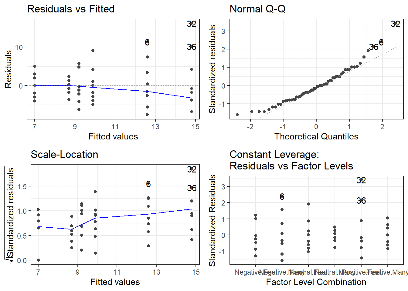

And if you feel as if you need it, use the leveneTest() function in the car package to get the Brown-Forsythe test (because levene’s apparently isn’t the default!)

This must be done at the cell means level, and leveneTest doesn’t play nice with Two-Way ANOVA models. You have to specify a formula with JUST the interaction term.

leveneTest(items ~ mood:stopRule, ocd)

Levene's Test for Homogeneity of Variance (center = median)
      Df F value Pr(>F)
group  5  1.7291 0.1436
      54