16  Generalized Linear Models

# Need the knitr package to set chunk options
library(knitr)
library(tidyverse)
library(gridExtra)
library(caret)
library(readr)

It should be noted that depending on the time frame that you may read about “GLMs”, this may refer to two different types of modeling schemes

• GLM \(\to\) General Linear Model: This is the older scheme that now refers to Linear Mixed Models or LMMs. This has more with correlated error terms and “random effects” in model.

• These days GLM refers to Generalized Linear Model. Developed by Nelder, John; Wedderburn, Robert (1972). This takes the concept of a linear model and generalizes it to response variables that do not have a normal distribution. This is what GLM means today. (I haven’t run into an exception, but there might be ones out there depending on the discipline.)

16.1 Components of Linear Model

We will start with the idea of the regression model we have been working.

\[ \mu_{y|x}= \beta_0 + \beta_1 x_1 + \beta_2 x_2 + \dots + \beta_p x_p. \]

• Here we are saying that the mean value of \(y\), \(\mu_{y|x}\), is determined by the values of our predictor variables.

• For making predictions, we have to add in a random component (because no model is perfect).

\[ y = \mu_{y|x} + \epsilon = \beta_0 + \beta_1 x_1 + \beta_2 x_2 + \dots + \beta_p x_p + \epsilon. \]

We have two components here.

1. A deterministic component.

2. A random component: \(\epsilon \sim N(0, \sigma^2)\).

• The random component means that \(Y \sim N(\mu_{y|x}, \sigma^2)\).

• The important part here is that the mean value of \(y\) is assumed to be linearly related to our \(x\) variables.

16.1.1 Introduction to Link Functions

We have tried transformations on data to try to see if we can fix heterogenity and non-linearity issues.

• In Generalized Linear Models these are known as link functions.
• The functions are meant to link a linear model to the distribution of \(y\) or link the distribution of \(y\) to a linear model. (which ever way you want to think about it)
• In the case of linear regression they are supposed to be the link of \(y\) with Normality and linearity.

Example:

\[ \begin{aligned} g(y) &= \log(y) &= \eta_{y|x} + \epsilon = \beta_0 + \beta_1 x_1 + \beta_2 x_2 + \dots + \beta_p x_p + \epsilon \end{aligned} \]

What does this mean for \(y\) itself?

\[ \begin{aligned} Y &= g^{-1}\left( \eta_{y|x} + \epsilon \right) = e^{\eta_{y|x}+ \epsilon}\\ \mu_{y|x} &= e^{\beta_0 + \beta_1 x_1 + \beta_2 x_2 + \dots + \beta_p x_p + \epsilon} \end{aligned} \]

• Another common option is \(g(Y) = Y^p\) where it could be hoped that \(p = 1\) but more often the best \(p\) is not…

16.1.2 Form of Generalized Linear Models

The form of Generalized Linear Models takes the basic form:

• Observations of \(y\) are the result of some probability distribution whose mean (and potentially variance) are determined or correlated with certain “predictor”/x variables.

• The mean value of \(y\) is \(\mu_{y|x}\) and is not linearly related to \(x\), but via the link function it is, i.e., \[g(\mu_{y|x}) = \]

There are now three components we consider:

1. A deterministic component.

2. The probability distribution of \(y\) with some mean \(\mu_{y|x}\) and standard deviation (randomness) \(\sigma_{y|x}\).

• In ordinary linear regression the probability distribution for \(y\) was \[N(\beta_0 + \beta_1 x_1 + \beta_2 x_2 + \dots + \beta_p x_p, \sigma)\]
• Consider \(y\) from a binomial distribution with probability of success \(p(x)\), that is, the probability depends on \(x\). For an individual trial, we have:
  • \(\mu_{y|x} = p(x)\)
  • \(\sigma_{y|x} = \sqrt{p(x)(1-p(x))}\)
  • This makes is so we can no longer just chuck the error term into the linear equation for the mean to represent the randomness.

3. A link function \(g(y)\) such that

\[ \begin{aligned} g\left(\mu_{y|x}\right) &= \eta_{y|x}\\ &= \beta_0 + \beta_1 x_1 + \beta_2 x_2 + \dots + \beta_p x_p \end{aligned} \]

With GLMs, we are now paying attention to a few details.

• \(y\) is not restricted to the normal distributions; that’s the entire point…

• The link function is chosen based on the distribution of \(y\)

  • The distribution of \(y\) determines the form of \(\mu_{y|x}\).

16.1.3 Various Types of GLMs

Distribution of \(Y\)	Support of \(Y\)	Typical Uses	Link Name	Link Function: \(g(y)\)
Normal	\(\left(-\infty, \infty\right)\)	Linear response data	Identity	\(g\left(\mu_{y|x}\right) = \mu_{y|x}\)
Exponentail	\(\left(0, \infty\right)\)	Exponential Processes	Inverse	\(g\left(\mu_{y|x}\right) = \frac{1}{\mu_{y|x}}\)
Poisson	\(0,1,2,\dots\)	Counting	Log	\(g\left(\mu_{y|x}\right) = \log_{y|x}\)
Binomial	\(0,1\)	Classification	Logit	\(g\left(\mu_{y|x}\right) = \text{ln}\left(\frac{\mu_{y|x}}{1-\mu_{y|x}}\right)\)

We will mainly explore Logistic Regression, which uses the Logit function.

This is one of the ways of dealing with Classification.

16.2 Classification Problems, In General.

Classification can be simply define as determing what the outcome is for a discrete random variable.

• An online banking service must be able to determine whether or not a transaction being performed on the site is fraudulent, on the basis of the user’s past tranaction history, balance, an other potential predictors. This a common use of statistical classification known as Fraud detection

• On the basis of DNA sequence data for a number of patients with and without a given disease a biologist would like to figure out which DNA mutations are disease-causing and which are not.

• A person arrives at the emergency room with a set of symptoms that could possiblly be attributed to one of three medical conditions: stroke, drug overdose, epileptic seizure. We would want to choose or classify the person into one of the three categories.

In each of these situations what is the distribution of \(Y =\) the category an indidual falls into?

16.2.1 Odds and log-odds

In classification models, the idea to to estimate the probability of an event occuring for an individual: \(p\).

There are a couple of ways that we assess how likely an event is:

• Odds are \(Odds(p) = \frac{p}{1-p}\)
  • This is the ratio of an event occurring versus it not occurring.
  • This gives a numerical estimate of how many times more likely it is for the event to occur rather than not.
  • \(Odds = 1\) implies a fifty/fifty split: \(p = 0.5\). (Like a coin flip!)
  • \(Odds = d\) where \(d > 1\) implies that the event is \(d\) times more likely to happen than not.
  • For \(d < 0\) the event is \(1/d\) times more likely to NOT happen rather than happen.
• log-odds are taking the logarithm (typically the natural logarithm) of the odds: \(\log(Odds(p)) = log\left(\frac{p}{1-p}\right)\)$
  • In logistic regression, the linear relationship between \(p(x)\) and the predictor variables is assumed to be via \(\log(Odds)\).
  • \(log\left(\frac{p}{1-p}\right) = \beta_0 + \beta_1x_1 + \dots + \beta_kx_k\)

16.3 An Example, Default

We will consider an example where we are interested in predicting whether an individual will default on their credit card payment, on the basis of annual income, monthly credit card balance and student status. (Did I pay my bills… Maybe I should check.)

Default <- read_csv(here::here("datasets","Default.csv"))

# Converting Balance and Income to Thousands of dollars

Default$balance <- Default$balance/1000
Default$income <- Default$income/1000

head(Default)

# A tibble: 6 × 5
   ...1 default student balance income
  <dbl> <chr>   <chr>     <dbl>  <dbl>
1     1 No      No        0.730  44.4 
2     2 No      Yes       0.817  12.1 
3     3 No      No        1.07   31.8 
4     4 No      No        0.529  35.7 
5     5 No      No        0.786  38.5 
6     6 No      Yes       0.920   7.49

• student whether the person is a student or not.
• default is whether they defaulted
• balance is there total balance on their credit cards.
• income is the income of the individual.

16.3.1 A little bit of EDA

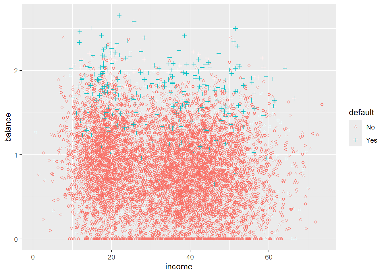
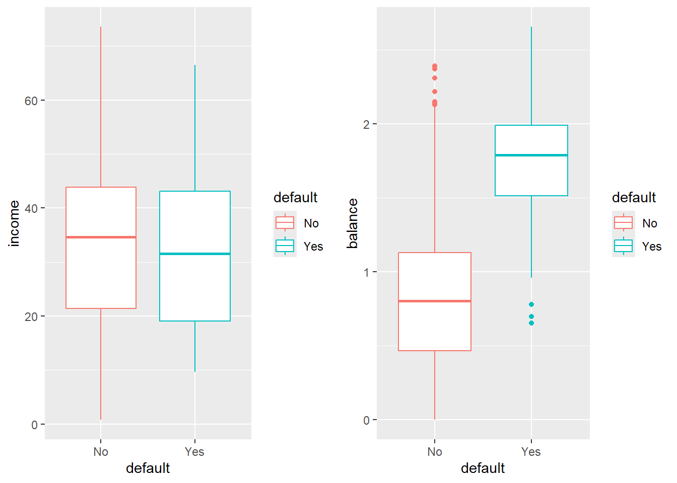
Try to describe what you see.

16.3.2 Logistic Regression

For each individual \(y_i\) we are trying to model if that individual is going to default or not.

• We will start by modeling \(P\text{(Default | Balance}) \equiv P(Y | x)\).

• First, we we will code the default to a 1, 0 format to make modeling this probability compatible with the standard form of the with a special case of the Binomial\((n,p\)) distribution where \(n =1\)

\[ P(Y = 1) = p(x) \]

• Logistic regression creates a model for \(P(Y=1|x)\) (technically the log-odds thereof) which we will abbreviate as \(p(x)\)

# Set an ifelse statement to handle the variable coding

#Create a new varible called def with the coded values
Default$def <- ifelse(Default$default == "Yes", 1,0)

Before we get into the actual Logistic Regression model, lets start with the idea that if we are trying to predict \(p(x)\), when should we should we say that someone is going to default?

• A possiblity may be we classify the person as potentially defaulting if \(p(x) > 0.5\)

• Would it make sense to predict somone as a risk for defaulting at some other cutoff?

16.3.3 Plotting

def.plot <- ggplot(Default, aes(x = balance, y = def, color = def)) + geom_point() +
  xlab("Balance") + ylab("Default")

def.plot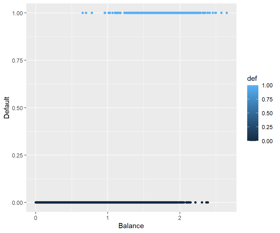

16.3.4 Why Not Linear Regression

We could use standard linear regression to model \(p(\text{Balance}) = p(x)\). The line on this plot represents the estimated probability of defaulting.

def.plot.lm <- ggplot(Default, aes(x = balance, y = def, color = def)) + geom_point()+
  xlab("Balance") + ylab("Default") +
  geom_smooth(method = 'lm')

def.plot.lm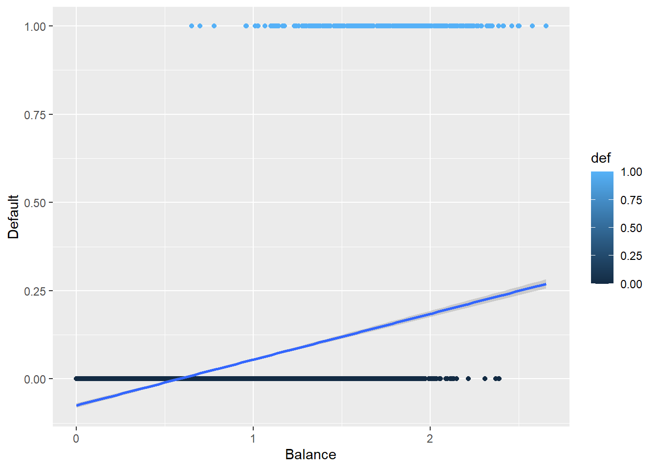

Can you think of any issues with this? Think about possible values of \(p(x)\).

16.3.5 Plotting the Logistic Regression Curve

Here is the curve for a logistic regression.

def.plot.logit <- ggplot(Default, aes(x = balance, y = def, color = def)) + geom_point() +
  xlab("Balance") + ylab("Default") +
  geom_smooth(method = "glm", method.args = list(family = "binomial"))
  
def.plot.logit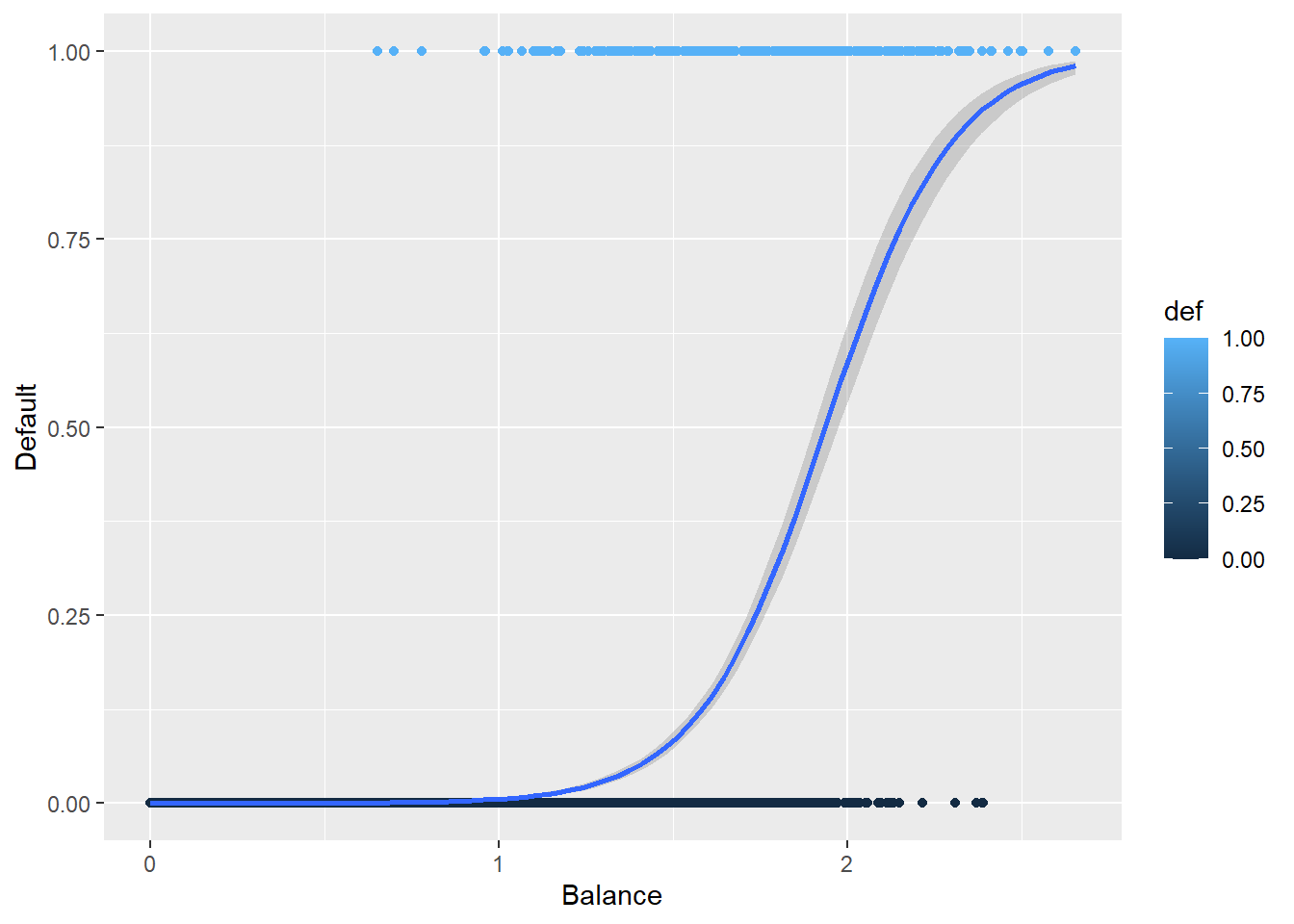

How does this compare to the previous plot?

16.4 The Logistic Model in GLM

Even though we are trying to model a \(p(x)\), we are trying to model a mean.

What is the mean or Expected Values of a binomial random variable \(Y|x \sim\) Binomial\((1, p(x))\)?

Before we get into the link function, lets look at the function that models \(p(x)\)

\[ p(x) = \dfrac{e^{\beta_0 + \beta_1x}}{1 + e^{\beta_0 + \beta_1x}} \]

The link functions for Logistic Regression is the logit function which is

\[ \text{logit}(x) = \log\left(\frac{m}{1-m}\right) \text{ where } 0<x<1 \]

Which for \(\mu_{y|x} = p(x)\) is

\[ \log\left( \frac{p(x)}{1-p(x)} \right) = \beta_0 + \beta_1 x \]

• Notice that now we have a linear function of the coefficients.

• Something to pay attention to: When we are interpreting the coefficients, we are talking about how the log odds change.

• The coefficients tell us what the percentage increase of the odds ratio would be.

\[ \text{Odds} = \frac{p(x)}{1-p(x)} \]

16.4.1 Estimating The Coefficients: glm function

The function that is used for GLMs in R is the glm function.

glm(formula, family = gaussian, data)

• formula: the linear formula you are using when the link function is applied to \(\mu(vx)\). This has same format as lm, e.g, y ~ x

• family: the distribution of \(Y\) which in logistic regression is binomial

• data: the dataframe… as has been the case before.

16.4.2 GLM Function on Default Data

default.fit <- glm(def ~ balance, family = binomial, data = Default)

summary(default.fit)

Call:
glm(formula = def ~ balance, family = binomial, data = Default)

Coefficients:
            Estimate Std. Error z value Pr(>|z|)    
(Intercept) -10.6513     0.3612  -29.49   <2e-16 ***
balance       5.4989     0.2204   24.95   <2e-16 ***
---
Signif. codes:  0 '***' 0.001 '**' 0.01 '*' 0.05 '.' 0.1 ' ' 1

(Dispersion parameter for binomial family taken to be 1)

    Null deviance: 2920.6  on 9999  degrees of freedom
Residual deviance: 1596.5  on 9998  degrees of freedom
AIC: 1600.5

Number of Fisher Scoring iterations: 8

16.4.3 Default Predictions

“Predictions” in GLM models get a bit trickier than previously.

• We can predict in terms of the linear response, \(g(\mu(x))\), e.g., log odds in logistic regression.

• Or we can predict in terms of the actual response variable, e.g., \(p(x)\) in logistic regression.

\[ \log\left(\frac{\widehat{p}(x)}{1-\widehat{p}(x)}\right) = -10.6513 + 5.4090x \]

Which may not be very useful in application.

log

So for someone with a credict balance of 1000 dollars, we would predict that their probability of defaulting is

\[ \widehat{p}(x) = \frac{e^{-10.6513 + 5.4090\cdot 1}}{1 + e^{-10.6513 + 5.4090 \cdot 1}} = 0.00526 \]

And for someone with a credit balance of 2000 dollars, our prediction probability for defaulting is

\[ \widehat{p}(x) = \frac{e^{-10.6513 + 5.4090\cdot 2}}{1 + e^{-10.6513 + 5.4090 \cdot 2}} = 0.54158 \]

16.5 Interpreting coefficients

Because of what’s going on in logistic regression, we have forms for our model:

1. The linear form which is for predicting log-odds.
2. Odds ratios which is the exponentiated form of the model, i.e., \(e^{\beta_0 + \beta_1x}\).

• Then, we look at odds increasing (positive \(\beta_1\)) or decreasing (negative \(\beta_1\)) by \(e^{\beta_1}\) times.

3. Probabilities which are of the form \(\frac{e^{\beta_0 + \beta_1x}}{1 + e^{\beta_0 + \beta_1x}}\).

• Then \(\beta_1\) means… Nothing really intuitive.
• You just say \(\beta_1\) indicates increasing or decreasing probability respective of whether \(\beta_1\) is postive or negative.

Honestly, GLMs are where interpretations get left behind because the link functions screw with our ability to make sense of the math.

16.6 Predict Function for GLMS

We can compute our predictions by hand but, that’s not super efficient. We can infact use the predict function on glm objects just like we did with lm objects.

With GLMs, our predict function now takes the form:

predict(glm.model, newdata, type)

• glm.model is the glm object you created to model the data.
• newdata is the data frame with values of your predictor variables you want predictions for. If no argument is given (or its incorrectly formatted) you will get the fitted values for your training data.
• type chooses which form of prediction you want.
  • type = "link" (the default option) gives the predictions for the link function, i.e, the linear function of the GLM. So for logistic regression it will spit out the predicted values of the log odds.
  • type = "response" gives the prediction in terms of your response variable. For Logistic Regression, this is the predicted probabilities.
  • type = "terms" returns a matrix giving the fitted values of each term in the model formula on the linear predictor scale. (idk)

16.6.1 Using predict on Default Data

Let’s get predictions from the logistic regression model that’s been created.

predict(default.fit, newdata = data.frame(balance = c(1,2)), type = "link")

         1          2 
-5.1524137  0.3465032 

predict(default.fit, newdata = data.frame(balance = c(1,2)), type = "response")

          1           2 
0.005752145 0.585769370 

16.6.2 Classifying Predictions

If we are looking at the log odds ratio, we will classify an observation as a \(\widehat{Y}= 1\) if the log odds is non-negative.

Default$pred.link <- predict(default.fit)
Default$pred.class1 <-as.factor(ifelse(Default$pred.link >=0, 1, 0))

Or we can classify based off the predicted probabilities, i.e., \(\widehat{Y} = 1\) if \(\widehat{p}(x) \geq 0.5\).

Default$pred.response <- predict(default.fit, type = "response")
Default$pred.class2 <-as.factor(ifelse(Default$pred.response >=0.5, 1, 0))

Which will produce identical classifications.

sum(Default$pred.class1 != Default$pred.class2)

[1] 0

16.6.3 Assessing Model Accuracy

We can assess the accuracy of the model using a confusion matrix using the confusionMatrix function, which is part of the caret package.

• Note that this will require you to install the e1071 package (which I can’t fathom why they would do it this way…).

confusionMatrix(Predicted, Actual)

confusionMatrix(Default$pred.class1, as.factor(Default$def))

Confusion Matrix and Statistics

          Reference
Prediction    0    1
         0 9625  233
         1   42  100
                                          
               Accuracy : 0.9725          
                 95% CI : (0.9691, 0.9756)
    No Information Rate : 0.9667          
    P-Value [Acc > NIR] : 0.0004973       
                                          
                  Kappa : 0.4093          
                                          
 Mcnemar's Test P-Value : < 2.2e-16       
                                          
            Sensitivity : 0.9957          
            Specificity : 0.3003          
         Pos Pred Value : 0.9764          
         Neg Pred Value : 0.7042          
             Prevalence : 0.9667          
         Detection Rate : 0.9625          
   Detection Prevalence : 0.9858          
      Balanced Accuracy : 0.6480          
                                          
       'Positive' Class : 0               
                                          

16.7 Categorical Predictors

Having categorical variables and including multiple predictors is pretty easy. It’s just like with standard linear regression.

Let’s look at the model that just uses the student variable to predict the probability of defaulting.

default.fit2 <- glm(def ~ student,
                    family = binomial,
                    data = Default)

summary(default.fit2)

Call:
glm(formula = def ~ student, family = binomial, data = Default)

Coefficients:
            Estimate Std. Error z value Pr(>|z|)    
(Intercept) -3.50413    0.07071  -49.55  < 2e-16 ***
studentYes   0.40489    0.11502    3.52 0.000431 ***
---
Signif. codes:  0 '***' 0.001 '**' 0.01 '*' 0.05 '.' 0.1 ' ' 1

(Dispersion parameter for binomial family taken to be 1)

    Null deviance: 2920.6  on 9999  degrees of freedom
Residual deviance: 2908.7  on 9998  degrees of freedom
AIC: 2912.7

Number of Fisher Scoring iterations: 6

predict(default.fit2, 
        newdata = data.frame(student = c("Yes", 
                                         "No")), 
        type = "response")

         1          2 
0.04313859 0.02919501 

Would student status by itself be useful for classifying individuals as defaulting or no?

16.8 Multiple Predictors

Similarly (Why isn’t there an ‘i’ in that?) to categorical predictors we can easily include multiple predictor variables. Why? Because with the link function, we are just doing linear regression.

\[ p_{y|x} = \dfrac{e^{\beta_0 + \beta_1x_1 + \beta_2x_2 \dots + \beta_px_p}}{1 + e^{\beta_0 + \beta_1x_1 + \beta_2x_2 \dots + \beta_px_p}} \]

The link functions is still the same.

\[ \text{logit}(m) = \log\left(\frac{m}{1-m}\right) \text{ where } 0<x<1 \]

Which for \(\mu_{y|x} = p_{y|x}\) is

\[ \log\left( \frac{p_{y|x}}{1-p_{y|x}} \right) = \beta_0 + \beta_1x_1 + \beta_2x_2 \dots + \beta_px_p \]

16.8.1 Multiple Predictors in Default Data

Lets look at how the model does with using balance, income, and student as the predictor variables.

default.fit3 <- glm(def ~ balance + income + student, family = binomial, data = Default)

summary(default.fit3)

Call:
glm(formula = def ~ balance + income + student, family = binomial, 
    data = Default)

Coefficients:
              Estimate Std. Error z value Pr(>|z|)    
(Intercept) -10.869045   0.492256 -22.080  < 2e-16 ***
balance       5.736505   0.231895  24.738  < 2e-16 ***
income        0.003033   0.008203   0.370  0.71152    
studentYes   -0.646776   0.236253  -2.738  0.00619 ** 
---
Signif. codes:  0 '***' 0.001 '**' 0.01 '*' 0.05 '.' 0.1 ' ' 1

(Dispersion parameter for binomial family taken to be 1)

    Null deviance: 2920.6  on 9999  degrees of freedom
Residual deviance: 1571.5  on 9996  degrees of freedom
AIC: 1579.5

Number of Fisher Scoring iterations: 8

predict(default.fit3, 
        newdata = data.frame(balance = c(1,2), 
                             student = c("Yes",
                                         "No"), 
                             income=40),
        type = "response")

          1           2 
0.003477432 0.673773774 

predict(default.fit3, 
        newdata = data.frame(balance = c(1), 
                             student = c("Yes", 
                                         "No"), 
                             income=c(10, 50)),
        type = "response")

          1           2 
0.003175906 0.006821253