# Here are the libraries I used
library(tidyverse) # standard
library(knitr)
library(readr)
library(ggpubr) # allows for stat_cor in ggplots
library(ggfortify) # Needed for autoplot to work on lm()
library(gridExtra) # allows me to organize the graphs in a grid
library(car) # need for some regression stuff like vif
library(GGally)
library(mosaic) # For nicer TukeyHSD function that works with lm()13 ANOVA Assumptions
Here are some code chunks that setup this chapter.
# This changes the default theme of ggplot
old.theme <- theme_get()
theme_set(theme_bw())
13.1 Notation Reminder
\(y_{ij}\) is the \(j^{th}\) observation in the \(i^{th}\) treatment group.
- \(i = 1, \dots, t\), where \(t\) is the total number of treatment groups.
- \(j = 1, \dots, n_i\) where \(n_i\) is the number of observations in treatment group \(i\).
\(\overline{y}_{i.} = \sum_{j=1}^{n_i}\frac{y_ij}{n_i}\) is the mean of treatment group \(i\).
\(\bar{y}_{..} = \sum_{i=1}^{t} \sum_{j=1}^{n_i}\frac{y_{ij}}{N}\) is the over all mean of all observations.
- \(N\) is the total number of observations.
13.2 Assumptions
In ANOVA, we have the same assumptions. They have to do with the residuals!
Before the residuals in linear regression were:
\[e_i = y_{i} - \widehat{y}_{i}\]
Well now, an observations is \(y_{ij}\) and the any observation would best be predicted by its group mean \(\overline{y}_i\)
\[e_i = y_{ij} - \overline{y}_{i.}\]
- We assume the residuals are still normally distributed.
- The variability is constant between groups.
- Denote the standard deviation of population group \(i\) with \(\sigma_i\).
- We assume \(\sigma_1 = \sigma_2 = \dots = \sigma_t\).
- We assume they are independent. This is an issue in the situation where measurements are recorded over time.
- In linear regression, we additionally had to worry about model bias.
- This is not an issue in ANOVA.
- This is because we are estimating group means using sample means. Sample means are unbiased estimators by their very nature.
13.3 Checking them is about the same! autoplot()
oasis <- read_csv(here::here("datasets",
                             'oasis.csv'))
fit.lm <- aov(nWBV ~ Group, oasis)
autoplot(fit.lm)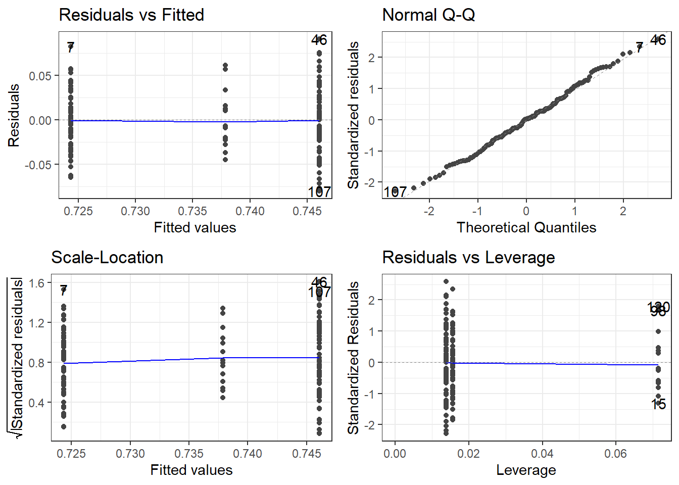
oasis %>%
  group_by(Group) %>%
  summarise(SD = sd(nWBV),
            Mean = mean(nWBV),
            n = length(nWBV))
# A tibble: 3 × 4
Group SD Mean n
<chr> <dbl> <dbl> <int>
1 Converted 0.0330 0.738 14
2 Demented 0.0315 0.724 64
3 Nondemented 0.0387 0.746 72The variability looks a bit smaller in the middle group, i.e., the Converted group. HOWEVER, that is only because there are so few observations in that group.
The normality looks pretty good.
13.3.1 Testing for Constant Variability/Homoskedasticity: Levene’s Test and Brown-Forsythe Test
To test for for constant variability in ANOVA, we use ANOVA.
The hypotheses are
\(H_0: \sigma_1 = \sigma_2 = \dots = \sigma_t\) \(H_1:\) At least one difference exists.
Instead of using the observations \(y_{ij}\), we use
\[z_{ij} = |y_{ij} - \overline y_{i.}|\]
or
\[z_{ij} = |y_{ij} - \tilde y_{i.}|\]
where \(\tilde y_{i.}\) is the median of a group.
- We call it Levene’s Test when using the mean \(\overline y_{i.}\) to compute \(z_{ij}\).
- We call it the Brown-Forsythe Test when using the median \(\tilde y_{i}\) to compute \(z_{ij}\).
Then the ANOVA process is used to to see if the mean of the \(z\) values differ between the groups.
- \(SST^* = \sum^n_{i=1} n_i\left(\overline z_{i.} - \overline z_{..}\right)^2\)
- \(SSE^* = \sum^n_{i=1} \left(z_{ij} - \overline z_{i.}\right)^2\)
\(\overline z_{i.}\) and \(\overline z_{..}\) are the group means and overall mean of the \(z_{ij}\)’s.
And then we have the mean squares. Just as before.
- \(MST^* = SST/(t-1)\)
- \(MSE^* = SSE/(N-t)\)
And our test statistic is
\[F^*_t = MST^*/MSE^*\]
- Under the null hypothesis this test statistic followsan \(F(t-1, N-t)\) distribution which is used to compute its p-value.
FYI: In many texts that I have seen, it is sometimes referred to as \(W\) instead of \(F_t^*\).
13.3.2 Levene/Brown-Forsythe in R
You need the car library and the function for performing either the Levene or Brown-Forsythe in R is leveneTest()
You only need one argument, your lm() or aov() depending on how you do the ANOVA:
leveneTest(model)- Despite its name, it is doing the Brown-Forsythe version of the test by default.
- To do the Levene Test, you have to specify a
centerargument.center = medianis Brown-Forsythe by default.center = meanis Levene.- So to perform Levene’s Test:
leveneTest(model, center = mean)
13.3.3 Oasis Example
fit.aov <- aov(formula = nWBV ~Group,
               data=oasis)


car::leveneTest(fit.aov)
Levene's Test for Homogeneity of Variance (center = median)
Df F value Pr(>F)
group 2 1.0268 0.3607
147 You may see some sort of warning message like:
Warning message:
In leveneTest.default(y = y, group = group, ...) : group coerced to factor.
Technically, the group variable should be a “factor” type of variable in R. This is just telling your grouping variable isn’t a “factor” type of variable and the function is assuming that it should be a “factor”.
leveneTest works on both the aov() and lm() model types.
13.4 What if the assumptions are violated?
Should normality be a major issue, then either transformations should be attempted or you should look into something called the Kruskal-Wallis test. And probably consult a statistician.
If the variability is not constant across groups, then there is Welch version of the ANOVA test.
To perform the Welch ANOVA, you would use the oneway.test().
You input just like with lm() or aov().
oneway.test(nWBV ~ Group, oasis)
    One-way analysis of means (not assuming equal variances)

data:  nWBV and Group
F = 6.4889, num df = 2.000, denom df = 37.508, p-value = 0.003801
Compare that to the standard ANOVA:
summary(fit.aov) Df Sum Sq Mean Sq F value Pr(>F)
Group 2 0.01601 0.008007 6.443 0.00208 **
Residuals 147 0.18268 0.001243
---
Signif. codes: 0 '***' 0.001 '**' 0.01 '*' 0.05 '.' 0.1 ' ' 1There is not much of a difference since the Brown-Forsythe test did not indicate there was reason to conclude the variability isn’t constant.
13.4.1 Games-Howell Procedure
The Games-Howell procedure is used to do pairwise comparisons when normality is not an issue but homogeneity is a concern.
- It is available via the
rstatixpackage. - Use the
games_howell_text()function.
The format is games_howell_test(data, formula, conf.level = 0.95, detailed = FALSE).
data: a data.frame containing the variables in the formula.formula: a formula of the form x ~ group where x is a numeric variable giving the data values and group is a factor with one or multiple levels giving the corresponding groups. For example,formula = TP53 ~ cancer_group.conf.level: confidence level of the interval.detailed: logical value. Default is FALSE. If TRUE, a detailed result is shown.
This package intends to change the paradigm of functions such that they are formatted so that the data argument is first. This is meant for compatibility with newer data-sciency uses of R that involve things called “pipes”
13.5 Some Extra Remarks
From this ResearchGate question.
Bruce Weaver writes what I consider to be some rather nice advice.
The numbered parts are verbatim from that link:
Levene’s test is a test of homogeneity of variance, not normality.
Testing for normality as a precursor to a t-test or ANOVA is not very helpful, IMO. Normality (within groups) is most important when sample sizes are small, but that is when tests of normality have very little power to detect non-normality. As the sample sizes increase, the sampling distribution of the mean converges on the normal distribution, and normality of the raw scores (within groups) becomes less and less important. But at the same time, the test of normality has more and more power, and so will detect unimportant departures from normality.
Rather than testing for normality, I would ask if it is fair and reasonable to use means and SDs for description. If it is, then ANOVA should be fairly valid.
Many authors likewise do not recommend testing for homogeneity of variance prior to doing a t-test or ANOVA. Box said that doing a preliminary test of variances was like putting out to sea in a row boat to see if conditions are calm enough for an ocean liner. I.e., he was saying that ANOVA is very robust to heterogeneity of variance. That is especially so when the sample sizes are equal (or nearly so). But as the sample sizes become more discrepant, heterogeneity of variance becomes more problematic. When sample sizes are reasonably similar, some authors suggest that ANOVA is robust to heterogeneity of variance so long as the ratio of largest variance to smallest variance is no more than 5:1.
However, let me add a note:
- It may not necessarily be useful to test for homogeneity of variability (and other assumptions), but it is good to inspect plots of the assumptions. If there is a huge discrepancy, then you’re going to want to address them.
13.5.1 One Final Note: Sample Sizes
Hopefully you end up taking a class in “Experimental Design”.
- There will be an emphasis on experiments with “balanced” data, i.e., each group has equal sample size.
- Often this will be impossible.
- Especially in experiments involving people.
- I have tried to provide tools that are robust alternatives.
- A caveat is that if you have extremely unbalanced samples, e.g., 5 in one group and 50 in another group.
- You should be very careful and probably need to learn new methods or consult a statistician.