# Here are the libraries I used
library(tidyverse) # standard
library(knitr) # need for a couple things to make knitted document to look nice
library(readr) # need to read in data
library(ggpubr) # allows for stat_cor in ggplots
library(ggfortify) # Needed for autoplot to work on lm()
library(gridExtra) # allows me to organize the graphs in a grid
library(car)8 Introduction to Multiple Regression
Here are some code chunks that setup this chapter
# This changes the default theme of ggplot
old.theme <- theme_get()
theme_set(theme_bw())
8.1 SENIC Data
We will now begin the examining data from the Study on the Efficcacy of Nosocomial Infection Control (SENIC project). The general objective, and therefore project name, was to examine how effective infection surveillance and control programs were at reducing hopsital acquired (nosocomial) diseases. Data was obtained through the test Applied Linear Statistical Models 5th edition (Neter et al).
senic <- read_csv(here::here("datasets",
'SENIC.csv'))stayLength: Average length of stay of all patients in hospital (in days)age: Average age of patients (in years)infectionRisk: Average estimated probability of acquiring infection in hospital (in percent)cultureRatio: Ratio of number of cultures performed to number of patients without signs or symptoms of hospital-acquired infection, times 100xrayRatio: Ratio of number of X-rays performed to number of patients , without signs or symptoms of pneumonia, times 100beds: Average number of beds in hospital during study periodschoolMed school affiliation (Yes or No)region: Geographic region (NE, NC, S, W)patients: Average number of patients in hospital per day during study periodnurses: Average number of full-time equivalent registered and licensed practical nurses during study period (number full-time plus one half the number part time)facilities: Percent of 35 potential facilities and services that are provided by the hospital
8.2 Infection Risk
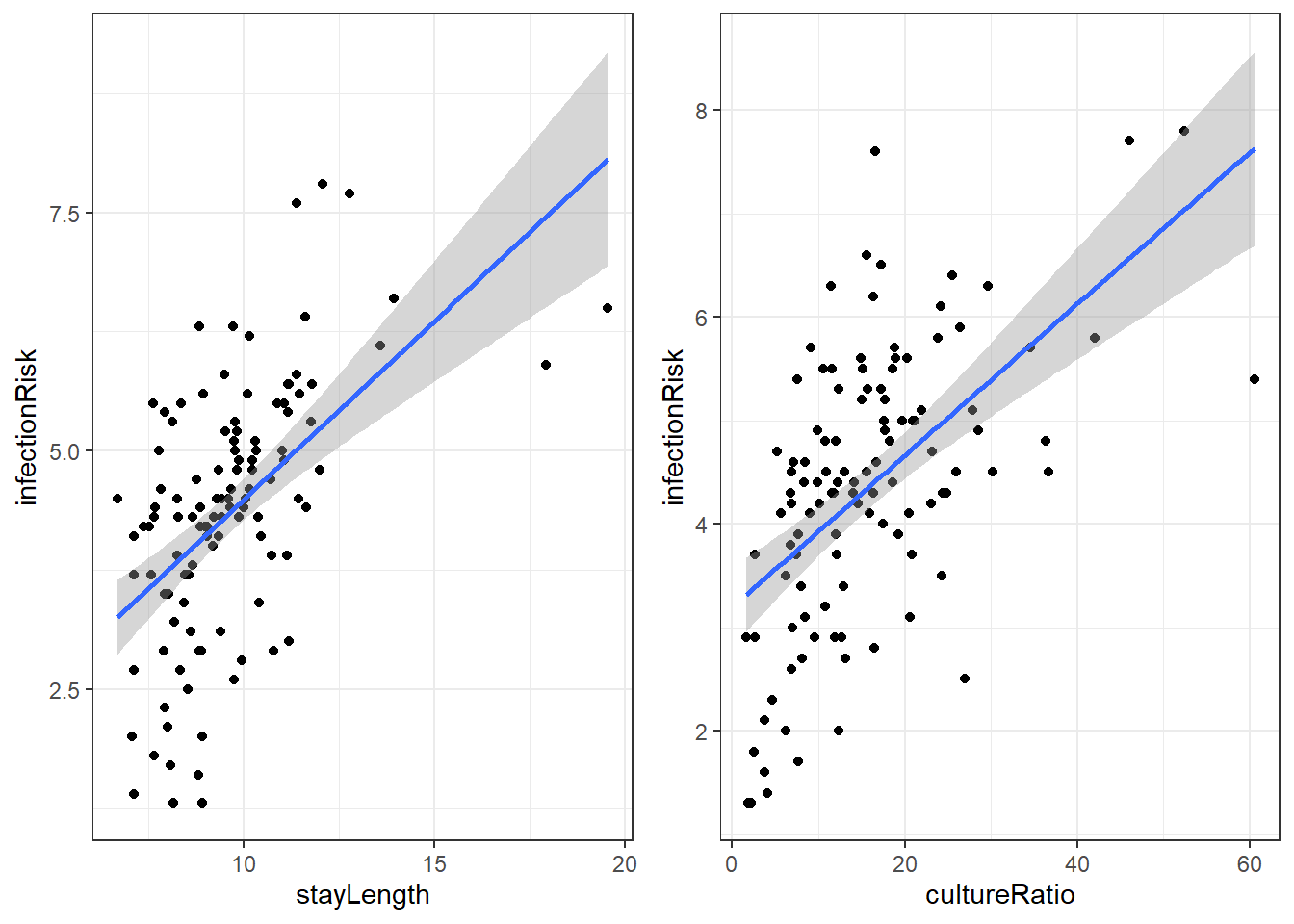
There are a lot of potential variables that may relate to infectionRisk, but let’s just concentrate on stayLength and cultureRatio.
#isc ending indicates the variables used:
#(i)nfectionRisk, (s)tayLength, (c)ultureRatio

senicisc <- select(senic, infectionRisk,
                   stayLength, cultureRatio)
8.2.1 Relation of infectionRisk with stayLength and cultureRatio
8.2.2 Model with stayLength
Here is the linear regression output for infectionRisk with stayLength.
infStayLm <- lm(infectionRisk ~ stayLength, senicisc)
summary(infStayLm)
Call:
lm(formula = infectionRisk ~ stayLength, data = senicisc)

Residuals:
    Min      1Q  Median      3Q     Max
-2.7823 -0.7039  0.1281  0.6767  2.5859

Coefficients:
            Estimate Std. Error t value Pr(>|t|)
(Intercept)  0.74430    0.55386   1.344    0.182
stayLength   0.37422    0.05632   6.645 1.18e-09 ***
---
Signif. codes:  0 '***' 0.001 '**' 0.01 '*' 0.05 '.' 0.1 ' ' 1

Residual standard error: 1.139 on 111 degrees of freedom
Multiple R-squared:  0.2846,    Adjusted R-squared:  0.2781
F-statistic: 44.15 on 1 and 111 DF,  p-value: 1.177e-09
Our regression equation for predicting infectionRisk is:
\[\widehat{risk} = 0.744 + 0.374\cdot stayLength\]
8.2.3 Model with cultureRatio
Here is the linear regression output for infectionRisk with cultureRatio.
infCuLm <- lm(infectionRisk ~ cultureRatio, senicisc)
summary(infCuLm)
Call:
lm(formula = infectionRisk ~ cultureRatio, data = senicisc)

Residuals:
    Min      1Q  Median      3Q     Max
-2.6759 -0.7133  0.1593  0.7966  3.1860

Coefficients:
             Estimate Std. Error t value Pr(>|t|)
(Intercept)   3.19790    0.19377  16.504  < 2e-16 ***
cultureRatio  0.07326    0.01031   7.106 1.22e-10 ***
---
Signif. codes:  0 '***' 0.001 '**' 0.01 '*' 0.05 '.' 0.1 ' ' 1

Residual standard error: 1.117 on 111 degrees of freedom
Multiple R-squared:  0.3127,    Adjusted R-squared:  0.3065
F-statistic: 50.49 on 1 and 111 DF,  p-value: 1.218e-10
The regression equation is then:
\[\widehat{risk} = 3.198 + 0.073\cdot cultureRatio\]
8.3 Linear Regression with Two Variables
We can “easily” create a model that accounts for a linear relationship between two variables. If we have one response variable \(y\) and two predictor variables \(x_1\) and \(x_2\), then the model is:
\[y = \beta_0 + \beta_1 x_1 + \beta_2 x_2 + \epsilon\]
Where we assume that we have error terms \(\epsilon \sim N(0,\sigma_\epsilon)\) which are independent. An additional assumption is that the two predictor variables, \(x_1\) and \(x_2\) are independent of each other.
We still have two parts to the model.
- The linear relation/conditional mean \(\mu_{y|x} = \beta_0 + \beta_1 x_1 + \beta_2 x_2\)
- The error \(\epsilon\)
8.4 Model for infectionRisk using two variables
The way to get the estimated regression equation is the same. We just add another variable into the lm() formula.
riskLm <- lm(infectionRisk ~ stayLength + cultureRatio,
             data=senicisc)

summary(riskLm)
Call:
lm(formula = infectionRisk ~ stayLength + cultureRatio, data = senicisc)

Residuals:
    Min      1Q  Median      3Q     Max
-2.1822 -0.7275  0.1040  0.6847  2.7143

Coefficients:
             Estimate Std. Error t value Pr(>|t|)
(Intercept)  0.805491   0.487756   1.651    0.102
stayLength   0.275472   0.052465   5.251 7.46e-07 ***
cultureRatio 0.056451   0.009798   5.761 7.70e-08 ***
---
Signif. codes:  0 '***' 0.001 '**' 0.01 '*' 0.05 '.' 0.1 ' ' 1

Residual standard error: 1.003 on 110 degrees of freedom
Multiple R-squared:  0.4504,    Adjusted R-squared:  0.4404
F-statistic: 45.07 on 2 and 110 DF,  p-value: 5.04e-15
So our model for estimated risk is
\[\widehat{risk} = 0.805 + 0.275 \cdot stayLength + 0.056\cdot cultureRatio\]
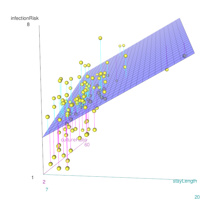
8.4.1 Graphing the relationship
8.4.2 Interpreting the Coefficients
The interpretation, so now we have to figure out to interpret three different estimated coefficients: \(\widehat \beta_{0}, \widehat \beta_{1}, \widehat \beta_{2}\).
\(\widehat \beta_{0}\) is the estimated y-intercept. The idea behind the intercept coefficient is similar, except for now it is \(\hat \mu_{y|x}hat\), the estimated mean value of the \(y\) variable, when both \(x_1\) and \(x_2\) are 0.
\(\widehat \beta_{1}\) is the amount that \(\hat \mu_{y|x}\) increases when \(x_1\) increases by 1 unit AND \(x_2\) is constant.
\(\widehat \beta_{2}\) is the amount that \(\hat \mu_{y|x}\) increases when \(x_2\) increases by 1 unit AND \(x_1\) is constant.
So for our estimated regression model:
\[\widehat{risk} = 0.805 + 0.275 \cdot stayLength + 0.056\cdot cultureRatio\]
We estimate that the mean infection risk of hospitals is 0.805% among hospitals with an average length of stay if 0 days and average culture ratio of 0. (Does this make sense?)
We estimate that the mean infection risk of hospitals increases by 0.275% among hospitals with average length of stay 1 day longer, and average culture ratio saying constant.
We estimate that the mean infection risk of hospitals increases by 0.056% among hospitals where the average culture ratio rate is 1 unit higher, and average length of stay remains constant.
8.5 Inference on the regression coefficients
Just like before, there are several columns for each coefficient. The columns are for the following hypothesis test.
\[H_0: \beta_k = 0\] \[H_1: \beta_k \ne 0\]
The test statistic is:
\[t = \frac{\hat \beta_k}{SE_{\hat \beta_k}}\]
We simple divide our coefficient estimate by its standard error.
The test statistic is assumed to be from a \(t\) distribution with degrees of freedom \(df = n - (p+1)\). Where \(p\) is the total number of predictor variables. And the p-value is the probability of obtaining
When looking at our model summary we interpret the p-values similarly.
summary(riskLm)
Call:
lm(formula = infectionRisk ~ stayLength + cultureRatio, data = senicisc)

Residuals:
    Min      1Q  Median      3Q     Max
-2.1822 -0.7275  0.1040  0.6847  2.7143

Coefficients:
             Estimate Std. Error t value Pr(>|t|)
(Intercept)  0.805491   0.487756   1.651    0.102
stayLength   0.275472   0.052465   5.251 7.46e-07 ***
cultureRatio 0.056451   0.009798   5.761 7.70e-08 ***
---
Signif. codes:  0 '***' 0.001 '**' 0.01 '*' 0.05 '.' 0.1 ' ' 1

Residual standard error: 1.003 on 110 degrees of freedom
Multiple R-squared:  0.4504,    Adjusted R-squared:  0.4404
F-statistic: 45.07 on 2 and 110 DF, p-value: 5.04e-15- There is weak evidence that the true linear model has a non-zero intercept.
- There is extremely strong evidence that there is a linear component in the relationship between
stayLengthandinfectionRisk(\(p<0.0001\)) whencultureRatiois included in the model. - There is extremely strong evidence that there is a linear component in the relationship between
cultureRatioandinfectionRisk(\(p<0.0001\)) whenstayLengthis included in the model.
The test for the intercept is not important (usually). The tests for the slopes are more important though not terribly so by themselves.
8.5.1 Confidence Intervals for Coefficients
We can likewise get confidence intervals for the coefficients. They take the general form:
\[\hat \beta_i \pm t_{\alpha/2, df} \cdot SE_{\hat \beta_i}\]
Again the \(t_{\alpha/2}\) quantile depends on the value for \(\alpha\) of the desired nominal confidence level \(1 - \alpha\).
To get the confidence intervals we use the confint() function just before.
confint(riskLm, level = 0.99) 0.5 % 99.5 %
(Intercept) -0.4730459 2.08402798
stayLength 0.1379482 0.41299604
cultureRatio 0.0307672 0.08213574The estimated change in the mean of infectionRisk is:
- From 0.138 to 0.413 at 99% confidence when increasing
stayLengthby 1 day. (And keepingcultureRatioconstant.) - From 0.031 to 0.082 at 99% confidence when increasing
cultureRatioby 1 (ratios don’t really have units). (KeepingstayLengthconstant.)
8.6 Estimating the Mean/Predicting Future Observations
Getting predictions is similar to before. You use the predict() function, and you need to specify what values you want predictions for.
You make a data.frame with values for each predictor variable.
- You must specify all variables that are used as predictors.
- Each variable must have the same number of points.
- If you screw this up, you will get predictions for all of the original points in the data.
Lets say you want to predict/estimate infectionRisk for a hospital that have an average length of stay of 5, 10, and 15 days, and a average culture ratio of 5, 15, 25. But which way are we combining those?
newdata <- data.frame(stayLength = c(5, 10, 15),
                      cultureRatio = c(5, 15, 25))
predict(riskLm, newdata)
1 2 3
2.465109 4.406984 6.348859 Or what about?
newdata <- data.frame(stayLength = c(5, 10, 15),
                      cultureRatio = c(25, 15, 5))
predict(riskLm, newdata)
1 2 3
3.594138 4.406984 5.219830 Or…?
newdata <- data.frame(stayLength = c(15, 5, 10),
                      cultureRatio = c(15, 25, 5))
predict(riskLm, newdata)
1 2 3
5.784345 3.594138 3.842469 You have to know which exact combination of predictor variable values you want.
8.6.1 Confidence Intervals for the Mean and Prediction Intervals for Future Observations
This is the same as well.
- Confidence intervals (CIs) are establishing a range of plausible values for the conditional mean: \(\mu_{y|x} = \beta_0 + \beta_1 x_1 + \widehat \beta_{2} x_2\)
- Prediction intervals (PIs) establish a range of plausible values for individual observations: \(y = \beta_0 + \beta_1 x_1 + \widehat \beta_{2} x_2 + \epsilon\)
Let’s make 99% CIs and PIs.
newdata <- data.frame(stayLength = c(15, 5, 10),
                      cultureRatio = c(15, 25, 5))
CIs <- predict(riskLm, newdata,
               interval = "confidence", level = 0.99)
PIs <- predict(riskLm, newdata,
               interval = "prediction", level = 0.99)
CIs fit lwr upr
1 5.784345 5.001363 6.567327
2 3.594138 2.803874 4.384403
3 3.842469 3.456304 4.228635PIs fit lwr upr
1 5.784345 3.0409109 8.527779
2 3.594138 0.8486173 6.339659
3 3.842469 1.1849346 6.500004Interpretations are now relative to the value of both predictors variables.
CI Interpretation: There is 99% confidence that the mean infection risk of hospitals with average length of stay of 15 days and culture ratio of 15 is between 5.00% to 6.57%.
PI Interpretation: There is 99% confidence that the infection risk of an Individual hospital with average length of stay of 15 days and culture ratio of 15 is between 3.04% to 8.53%.
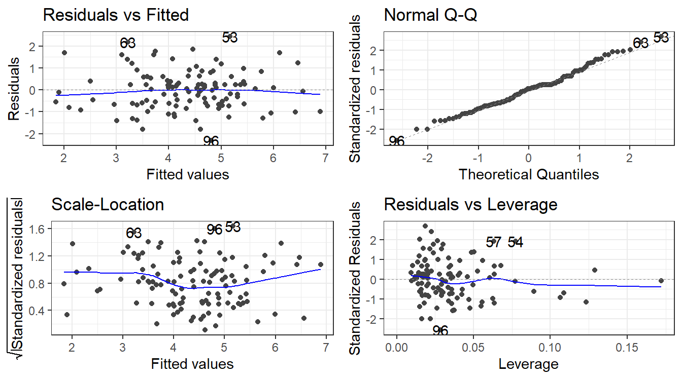
8.7 Residual Analysis
To assess validity of the model assumptions we can examine the residuals in the same manner as before. Create plots of the residuals using autoplot() and assess them in the same way as before.
autoplot(riskLm)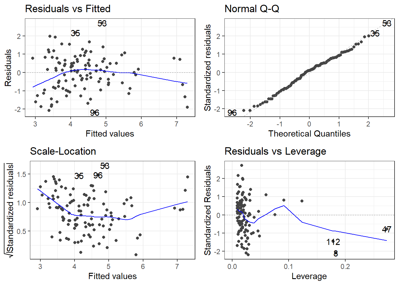
8.8 Adding more variables!
The linear model is not restricted to one or two variables. We can have as many predictor variables as we want! Let \(p\) denote the total number of predictor variables we use. The linear model is now:
\[y = \widehat \beta_0 + \widehat \beta_1 x_1 + \widehat \beta_{2} x_2 + ... + \widehat \beta_{p} + \epsilon = \beta_0 + \sum_{k=1}^p\beta_k x_k + \epsilon\]
8.8.1 facilities and infectionRisk?
Here is a graph between facilities and infectionRisk.
ggplot(senic, aes(x = facilities, y = infectionRisk)) +
  geom_point()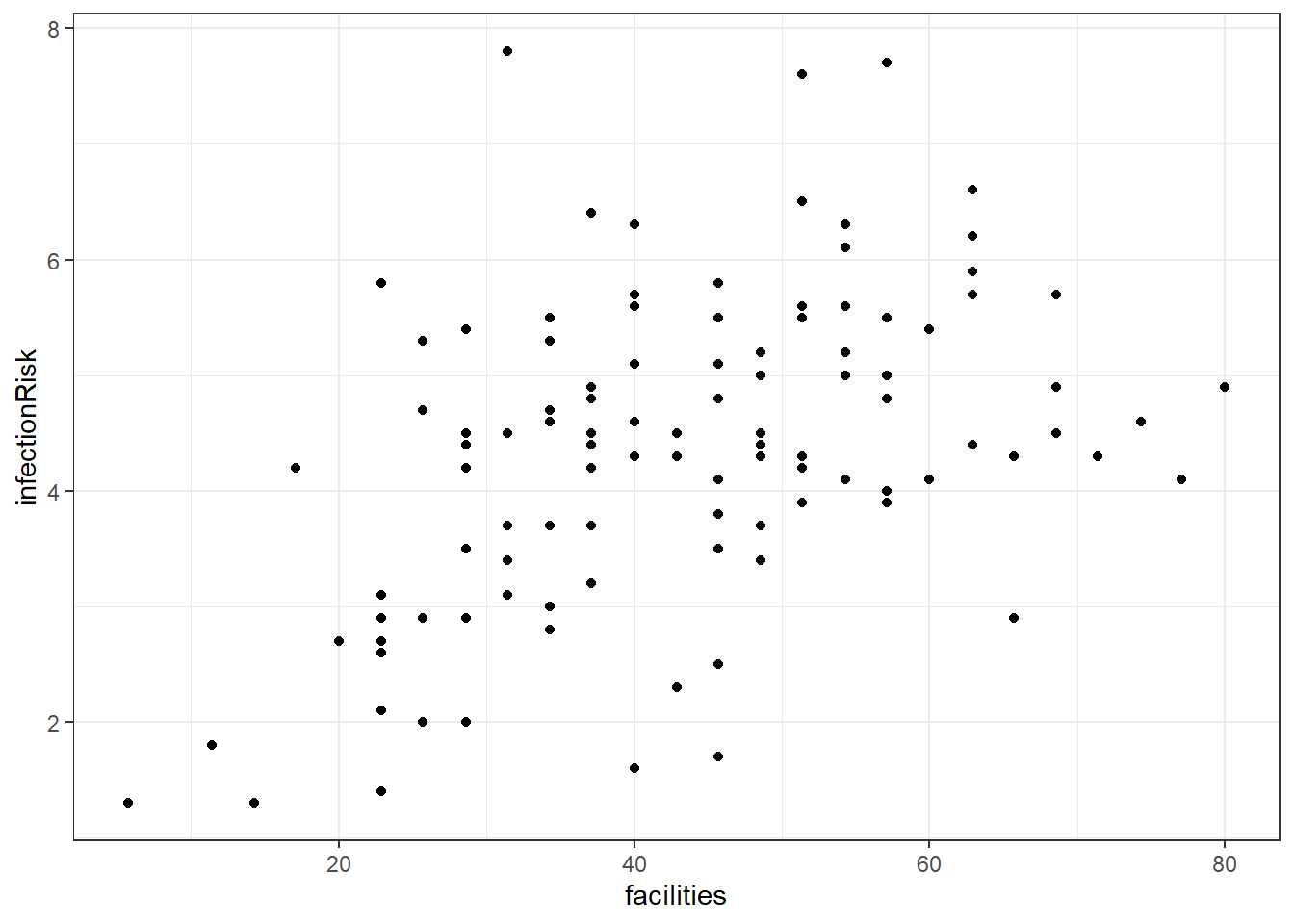
8.8.2 Adding facilities to the infectionRisk model.
riskierLm <- lm(infectionRisk ~ stayLength + cultureRatio + facilities, senic)
summary(riskierLm)
Call:
lm(formula = infectionRisk ~ stayLength + cultureRatio + facilities,
    data = senic)

Residuals:
     Min       1Q   Median       3Q      Max
-2.26400 -0.59873  0.01723  0.56650  2.64517

Coefficients:
             Estimate Std. Error t value Pr(>|t|)
(Intercept)  0.491332   0.481636   1.020  0.30992
stayLength   0.223907   0.053366   4.196 5.56e-05 ***
cultureRatio 0.054200   0.009479   5.718 9.55e-08 ***
facilities   0.019630   0.006454   3.042  0.00295 **
---
Signif. codes:  0 '***' 0.001 '**' 0.01 '*' 0.05 '.' 0.1 ' ' 1

Residual standard error: 0.9674 on 109 degrees of freedom
Multiple R-squared:  0.4934,    Adjusted R-squared:  0.4795
F-statistic: 35.39 on 3 and 109 DF,  p-value: 4.769e-16
8.8.3 Remember to always check your residuals!
autoplot(riskierLm)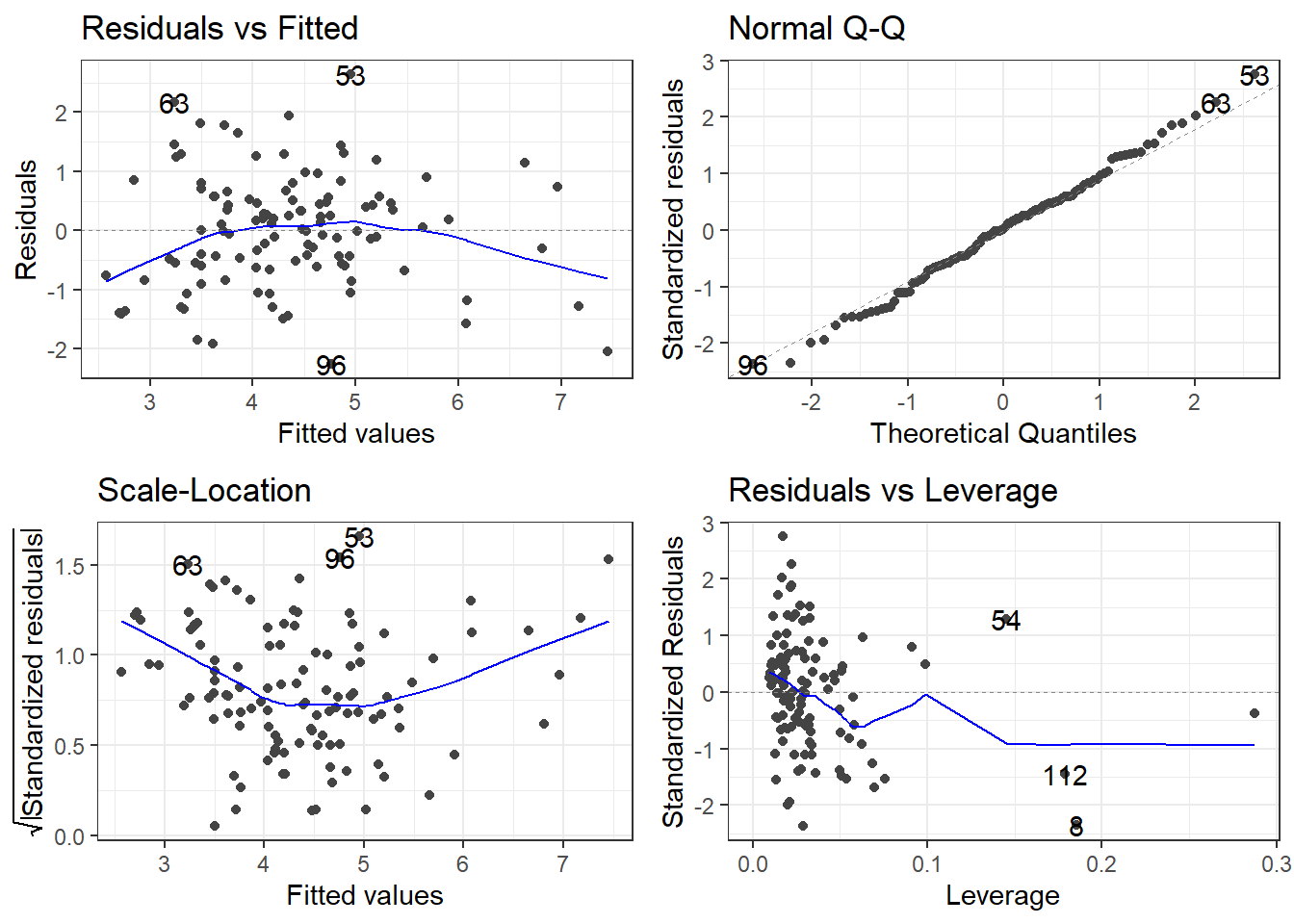
8.8.4 The Model Analysis of Variance: Global F-Test
Assuming there are \(p\) predictor variables
\(H_0: \beta_1 = \beta_2 = \dots = \beta_p = 0\)
\(H_1:\) At least one \(\beta_k\) is not \(0\).
To test this, we use that same breakdown of model variability as before:
\[SSTO = \sum_{i=1}^n(y_i - \bar y)^2\]
This variability in the variable can be broken up into two pieces:
\[SSR = \sum_{i=1}^n(\hat y_i - \bar y)^2 = \sum_{i=1}^n(\widehat \mu_{y|x} - \widehat\mu_y)^2\]
\[SSE = \sum_{i=1}^n(y_i - \widehat y_i)^2\]
The two sums of squares combined are the total variability \(SSTO\).
\[SSTO = SSR + SSE\] The Regression Degrees of Freedom is now \(p\), the error degrees of freedom is \(n - (p + 1)\).
This gives the following mean squares
- Mean Square Regression: \(MSR = SSR/p\)
- Mean Square Error: \(MSE = SSE/[n-(p+1)]\)
The test statistic is \(F_t = MSR/MSE\) and we use the \(F(p, n-(p +1))\) distribution to compute the p-value.
\[ F_t = \frac{SSR \div p}{MSE} = \frac{MSR}{MSE} \]
8.8.5 F-Test for infectionRisk model with 3 predictors
This test is available via the model summary in the very last row.
summary(riskierLm)
Call:
lm(formula = infectionRisk ~ stayLength + cultureRatio + facilities,
    data = senic)

Residuals:
     Min       1Q   Median       3Q      Max
-2.26400 -0.59873  0.01723  0.56650  2.64517

Coefficients:
             Estimate Std. Error t value Pr(>|t|)
(Intercept)  0.491332   0.481636   1.020  0.30992
stayLength   0.223907   0.053366   4.196 5.56e-05 ***
cultureRatio 0.054200   0.009479   5.718 9.55e-08 ***
facilities   0.019630   0.006454   3.042  0.00295 **
---
Signif. codes:  0 '***' 0.001 '**' 0.01 '*' 0.05 '.' 0.1 ' ' 1

Residual standard error: 0.9674 on 109 degrees of freedom
Multiple R-squared:  0.4934,    Adjusted R-squared:  0.4795
F-statistic: 35.39 on 3 and 109 DF,  p-value: 4.769e-16
Does this really matter? Ask yourself what the null hypothesis would and if it would matter.
8.8.6 Experiment: What happens to the stayLength slope?
Let’s look at the coefficients for the three models involving stayLength as a predictor.
By itself.
| term | estimate | std.error | statistic | p.value |
|---|---|---|---|---|
| (Intercept) | 0.7443037 | 0.5538573 | 1.343855 | 0.1817359 |
| stayLength | 0.3742169 | 0.0563195 | 6.644530 | 0.0000000 |
With cultureRatio.
coeff.summary(riskLm)| term | estimate | std.error | statistic | p.value |
|---|---|---|---|---|
| (Intercept) | 0.8054910 | 0.4877558 | 1.651423 | 0.1015044 |
| stayLength | 0.2754721 | 0.0524647 | 5.250615 | 0.0000007 |
| cultureRatio | 0.0564515 | 0.0097984 | 5.761279 | 0.0000001 |
And finally adding in facilities.
coeff.summary(riskierLm)| term | estimate | std.error | statistic | p.value |
|---|---|---|---|---|
| (Intercept) | 0.4913323 | 0.4816361 | 1.020132 | 0.3099249 |
| stayLength | 0.2239075 | 0.0533656 | 4.195726 | 0.0000556 |
| cultureRatio | 0.0542000 | 0.0094793 | 5.717698 | 0.0000001 |
| facilities | 0.0196303 | 0.0064539 | 3.041603 | 0.0029482 |
8.9 Transformations
A simple way to check the relationship between the variables would be to use the pairs() function. The pairs() function produces scatterplots between all variables you specify.
The basic syntax is pairs(formula, data) where formula is the formula of the regression model you are considering data is the dataset you are using.
pairs(infectionRisk ~ stayLength + cultureRatio + facilities,
      senic)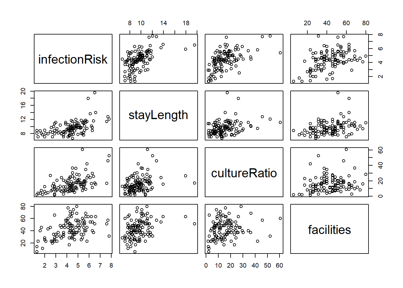
This is a scatterplot matrix. Notice that the vertical axis determined by the variable named to the left or right of a plot, and horizontal axis is determined by the variable named above or below a plot.
8.9.1 Finding the right transformations
pairs(infectionRisk ~ log(stayLength) +
        log(cultureRatio) +
        facilities, senic)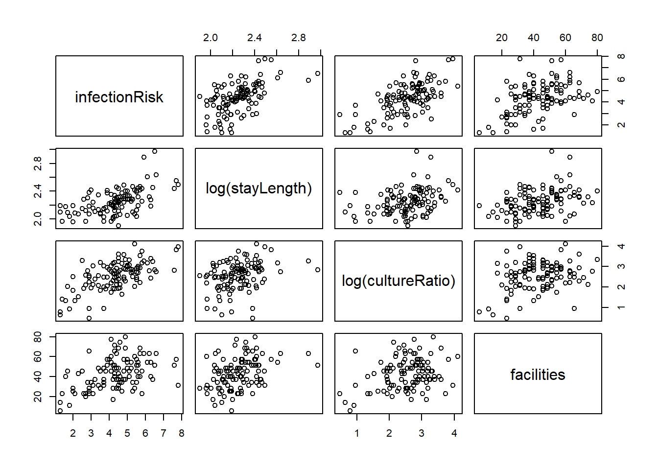
8.9.2 Incorporating them into the model
friskyLm <- lm(infectionRisk ~ log(stayLength) +
                 log(cultureRatio) +
                 facilities, senic)
summary(friskyLm)
Call:
lm(formula = infectionRisk ~ log(stayLength) + log(cultureRatio) +
    facilities, data = senic)

Residuals:
     Min       1Q   Median       3Q      Max
-2.31059 -0.63488  0.04808  0.54228  2.43225

Coefficients:
                   Estimate Std. Error t value Pr(>|t|)
(Intercept)       -4.255154   1.110040  -3.833 0.000212 ***
log(stayLength)    2.534644   0.540984   4.685 8.12e-06 ***
log(cultureRatio)  0.924657   0.134138   6.893 3.70e-10 ***
facilities         0.012736   0.006254   2.036 0.044147 *
---
Signif. codes:  0 '***' 0.001 '**' 0.01 '*' 0.05 '.' 0.1 ' ' 1

Residual standard error: 0.9138 on 109 degrees of freedom
Multiple R-squared:  0.548, Adjusted R-squared:  0.5355
F-statistic: 44.05 on 3 and 109 DF,  p-value: < 2.2e-16
8.9.3 Residuals!
autoplot(friskyLm)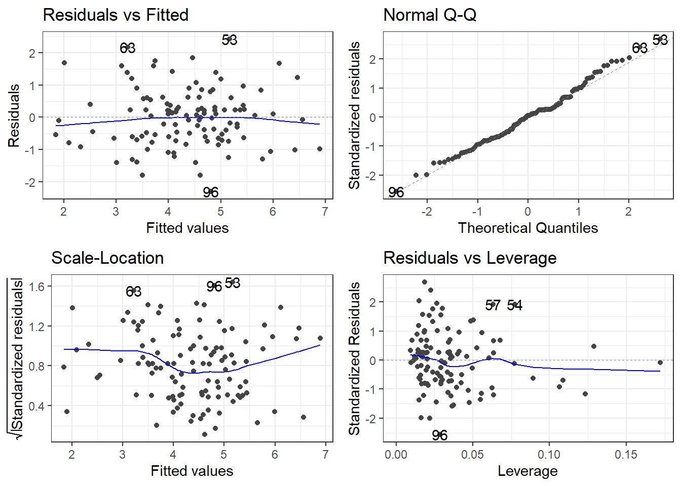
Then you have to reinterpret everything, and so on and so on.
8.9.4 Which log?
friskyLm2 <- lm(infectionRisk ~ log2(stayLength) +
                  log2(cultureRatio) +
                  facilities, senic)
summary(friskyLm2)
Call:
lm(formula = infectionRisk ~ log2(stayLength) + log2(cultureRatio) +
    facilities, data = senic)

Residuals:
     Min       1Q   Median       3Q      Max
-2.31059 -0.63488  0.04808  0.54228  2.43225

Coefficients:
                    Estimate Std. Error t value Pr(>|t|)
(Intercept)        -4.255154   1.110040  -3.833 0.000212 ***
log2(stayLength)    1.756881   0.374982   4.685 8.12e-06 ***
log2(cultureRatio)  0.640923   0.092977   6.893 3.70e-10 ***
facilities          0.012736   0.006254   2.036 0.044147 *
---
Signif. codes:  0 '***' 0.001 '**' 0.01 '*' 0.05 '.' 0.1 ' ' 1

Residual standard error: 0.9138 on 109 degrees of freedom
Multiple R-squared:  0.548, Adjusted R-squared:  0.5355
F-statistic: 44.05 on 3 and 109 DF,  p-value: < 2.2e-16
8.9.5 Can you spot the difference in residuals?
autoplot(friskyLm2)
autoplot(friskyLm)