# Here are the libraries I used
library(tidyverse) # standard
library(knitr) # need for a couple things to make knitted document to look nice
library(readr) # need to read in data
library(ggpubr) # allows for stat_cor in ggplots
library(ggfortify) # Needed for autoplot to work on lm()
library(gridExtra) # allows me to organize the graphs in a grid
library(car) # need for some regression stuff like vif
library(GGally)11 One-Way ANOVA
Here are some code chunks that setup this chapter.
# This changes the default theme of ggplot
old.theme <- theme_get()
theme_set(theme_bw())
Comparing More Than Two Group Means: Analysis of Variance (ANOVA or AOV)
11.1 Review: Comparing Two Groups (Sections 7.1 - 7.7 of JB Statistics)
Two-Sample Tests
\(H_0: \mu_1 = \mu_2\)
\(H_1: \mu_1 \neq \mu_2\)
11.1.1 The two-sample t-test: Pooled
Student’s two-sample \(t\)-test, and assumes unknown but equal population variances/standard deviations, i.e.,\(\sigma_1 = \sigma_2\).
We use a pooled sample variance estimate:
\[ s_p^2 = \frac{(n_1-1)s_1^2 + (n_2 - 1)s_2^2}{(n_1-1)+(n_2-1)} \]
\[ t = \frac{\bar{y_1}-\bar{y_2}}{\sqrt{s_P^2\left(\frac{1}{n_1}+\frac{1}{n_2}\right)}} \]
And the degrees of freedom is \(df = n_1 + n_2-2\)
Pro: Powerful if \(\sigma_1 = \sigma_2\).
Con: When is that true?
11.1.2 Welch’s two-sample t-test
Assume \(\sigma_1 \neq \sigma_2\) \[ t = \frac{\bar{y_1}-\bar{y_2}}{\sqrt{\frac{s_1^2}{n_1}+\frac{s_2^2}{n_2}}} \]
\[ df = \frac{\left(\frac{s_1^2}{n_1}+\frac{s_2^2}{n_2}\right)^2}{\frac{\left(s_1^2/n_1\right)^2}{n_1-1}+\frac{\left(s_2^2/n_2\right)^2}{n_2-1}} \]
11.1.3 R command, t.test()
t.test(x, y)By default, this performs Welch’s test. If you must perform Student’s test:
t.test(x, y, var.equal=TRUE)11.1.4 Hypothetical Example: Three Groups
Let’s consider having three groups.
In the code below, the groups are generated and technically we know the populations means.
But we will only have the sample data in reality.
How can we use three sample means at once to distinguish between three groups?
n = 200

data <- data.frame(x = rnorm(n, 0, 1),
                   y = rnorm(n, 1, 1), z = rnorm(n, 2, 1))
data <- gather(data, key = 'group', value = 'response')

# sample means

sample.means <- aggregate(x = response ~ group ,
                          data = data, FUN = mean)
sample.means$mu = c(0,1,2)

ggplot(data, aes(x = response, y = after_stat(density),
                 color = group, fill = group)) +
  geom_density(alpha = 0.5) +
  geom_vline(data = sample.means, aes(xintercept = response,
                                      color = group))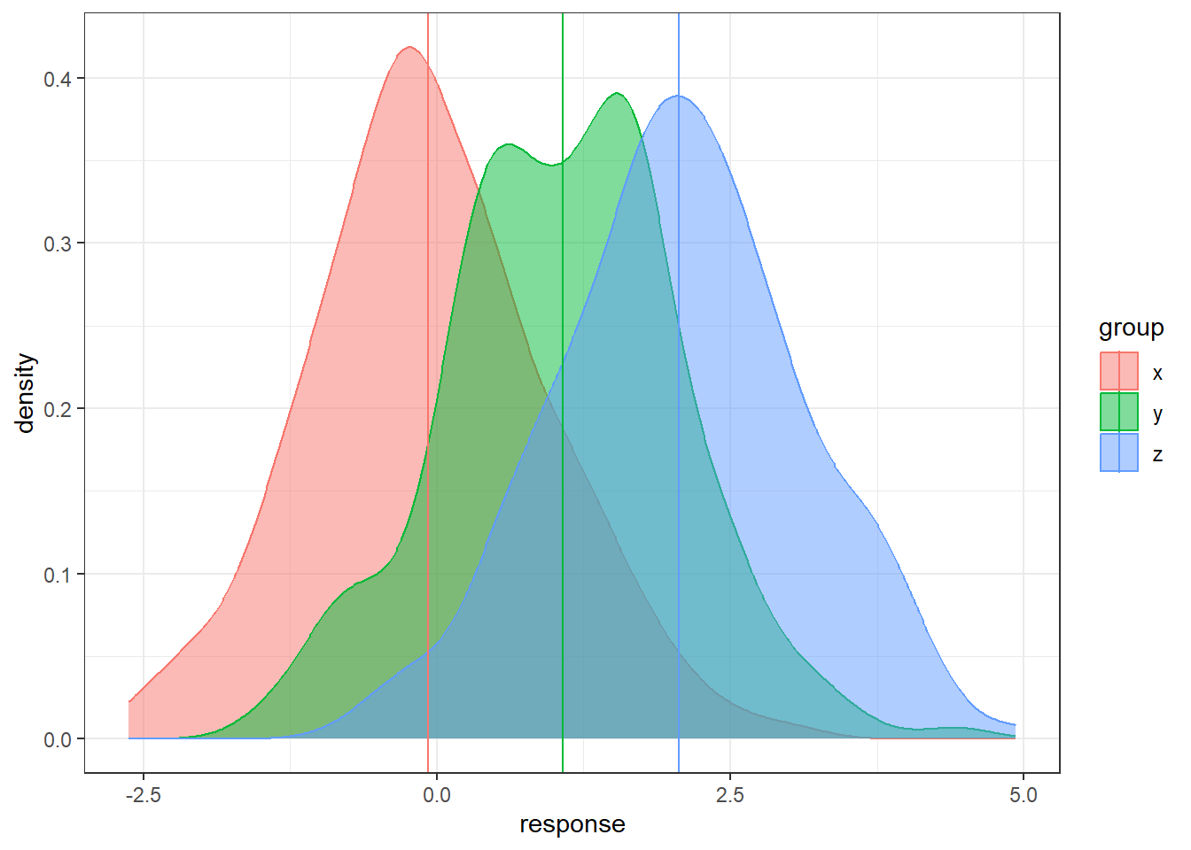
There is sampling variability associated with each sample mean. Run this code a few times do see how much the sample means will change from sample to sample. How do we account for the sampling variability when comparing three groups simultaneously? How do we even compare three groups simultaneously?
11.2 Analysis of Variance
11.2.1 General Objective of Analysis of Variance (ANOVA)
First, we are going to have a hypothesis test involved with comparing several groups.
The null hypothesis is going to be the similar to before, all the groups have equivalent population means.
The alternative is a bit trickier…
Hypotheses:
\(\begin{aligned} H_0&: \mu_1 = \mu_2 = \dots = \mu_t\\ H_1&: \text{not that...} \end{aligned}\)
Why not just do a bunch of separate t-tests?
If we have three groups:
- Compare group 1 to group 2.
- Compare group 1 to group 3.
- Compare group 2 to group 3.
And that would account for all possible pairings of groups. However, each of these would be a separate hypothesis test.
These are called pair-wise comparisons.
In general, if there are \(t\) groups, there are
\[\binom{t}{2} = \frac{t(t-1)}{2}\]
unique pair-wise comparisons.
11.2.2 Familywise Error Rate: What happens when you do multiple hypothesis tests
Say we had four treatment groups and we wanted to compare the means of all four groups to see if any differed.
Through pairwise comparisons, we would end up with \(\frac{4\cdot 3}{2} = 6\) total comparisons.
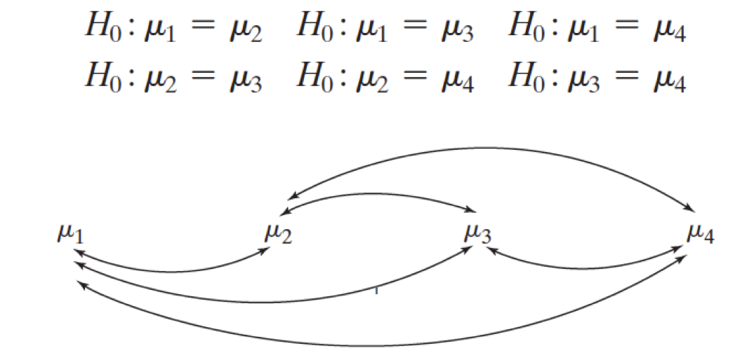
This would amount to 6 hypothesis tests to decide which if any group means differ.
- Assume each hypothesis test is done with the same Type I Error Rate \(\alpha\).
- Pr(Reject \(H_0\) | \(H_0\) True)
- This is known as a family of hypothesis tests, a set of hypothesis tests under one objective.
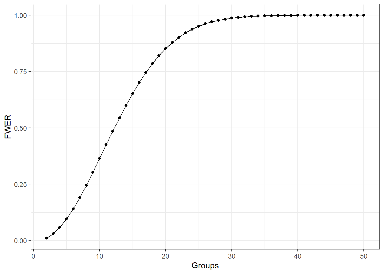
- The Family Wise Error Rate (FWER) is the probability of making at least one Type I Error among a family of hypothesis tests.
\[\begin{aligned} FWER & = 1 - (1 - \alpha)^c \\ &> \alpha \text{ for } c = 2, 3, \dots \end{aligned}\]
The following graph shows what happens to the FWER when the number of groups increases and each pairwise comparison done with \(\alpha = 0.01\).
11.2.3 How ANOVA Works
The analysis of variance (ANOVA) is just that. It looks at two types of variability in the data.
Between or Treatment Variability: This is the variability between the groups which is measured by essentially computing a the variance of the sample means between the different groups.
The Within or Error Variability: This is a collective measure of the variability within the groups.
If the Between/Treatment Variability is noticeably larger than the the Within/Error variability, we have strong evidence in favor that the least some groups have different population means.
11.2.4 Treatment versus Error Variability Demos
Here is a simulated dataset with moderately small within/error variability relative to the between/treatment variability
n = 200

data <- data.frame(x = rnorm(n, 0, 1),
                   y = rnorm(n, 1, 1), z = rnorm(n, 2, 1))
data <- gather(data, key = 'group', value = 'response')

sample.means <- aggregate(x = response ~ group ,
                          data = data, FUN = mean)
sample.means$mu = c(0,1,2)

ggplot(data, aes(x = response, y = after_stat(density),
                 color = group, fill = group)) +
  geom_density(alpha = 0.5) +
  geom_vline(data = sample.means, aes(xintercept = response,
                                      color = group))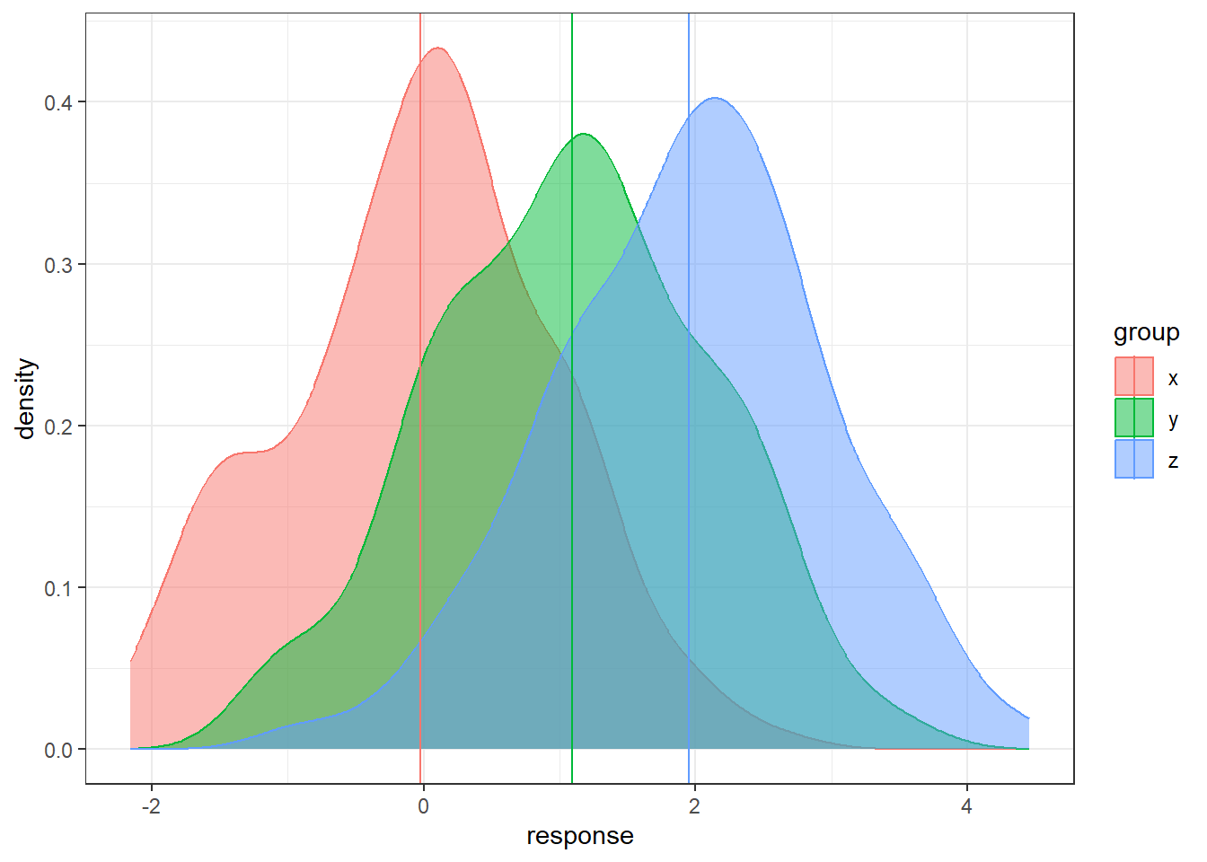
Here is an example a very small within/error variability relative to the between/treatment variability.
n = 200

data <- data.frame(x = rnorm(n, 0, 0.1),
                   y = rnorm(n, 1, 0.1), z = rnorm(n, 2, 0.1))
data <- gather(data, key = 'group', value = 'response')

# sample means

sample.means <- aggregate(x = response ~ group ,
                          data = data, FUN = mean)
sample.means$mu = c(0,1,2)

ggplot(data, aes(x = response, y = ..density..,
                 color = group, fill = group)) +
  geom_density(alpha = 0.5) +
  geom_vline(data = sample.means, aes(xintercept = response,
                                      color = group))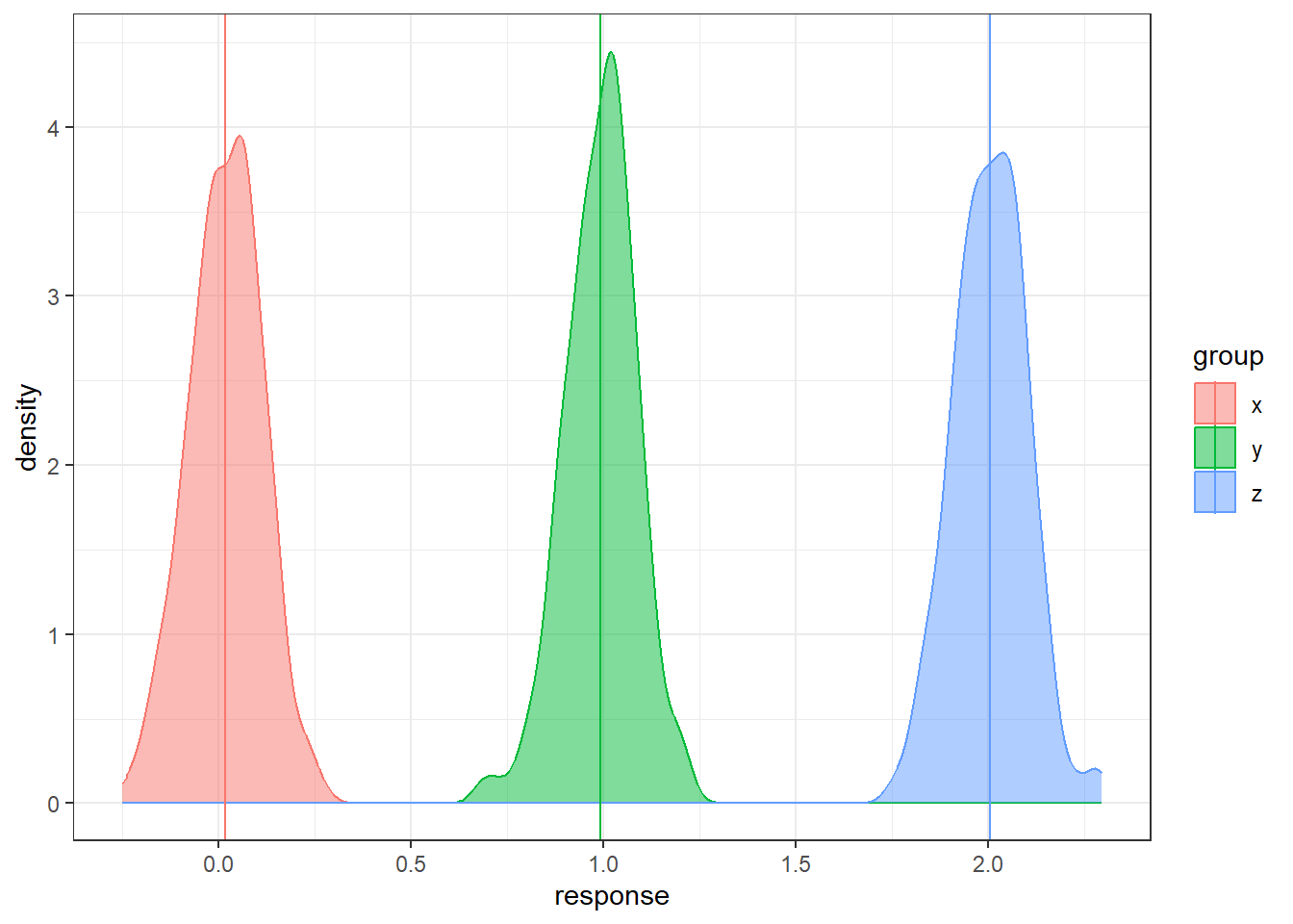
Lastly, large within/error variability relative to between/treatment variability.
n = 200

data <- data.frame(x = rnorm(n, 0, 5),
                   y = rnorm(n, 1, 5), z = rnorm(n, 2, 5))
data <- gather(data, key = 'group', value = 'response')

# sample means

sample.means <- aggregate(x = response ~ group ,
                          data = data, FUN = mean)
sample.means$mu = c(0,1,2)

ggplot(data, aes(x = response, y = ..density..,
                 color = group, fill = group)) +
  geom_density(alpha = 0.5) +
  geom_vline(data = sample.means, aes(xintercept = response,
                                      color = group))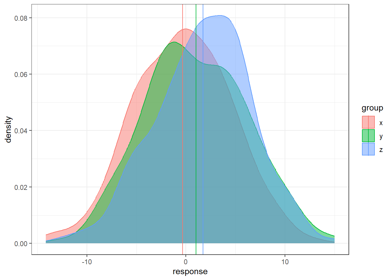
- In each situation, the population means are the same: 0, 1, and 2.
- In some situations it’s much easier to distinguish the groups than in others.
11.3 Formulating ANOVA: Notation
\(y_{ij}\) is the \(j^{th}\) observation in the \(i^{th}\) treatment group.
- \(i = 1, \dots, t\), where \(t\) is the total number of treatment groups.
- \(j = 1, \dots, n_i\) where \(n_i\) is the number of observations in treatment group \(i\).
\(\overline{y}_{i.} = \sum_{j=1}^{n_i}\frac{y_ij}{n_i}\) is the mean of treatment group \(i\).
\(\bar{y}_{..} = \sum_{i=1}^{t} \sum_{j=1}^{n_i}\frac{y_{ij}}{N}\) is the over all mean of all observations.
- \(N\) is the total number of observations.
11.3.1 Sums of Squares
Sum of Squares for the treatments
\(\begin{aligned} SST &= \sum_{i=1}^{t} n_i \left(\overline{y}_{i.} - \bar{y}_{..}\right)^2 \end{aligned}\)
Sum of squares for the errors
\(\begin{aligned} SSE &= \sum_{i=1}^{t} \sum_{j=1}^{n_i}\left(y_{ij} - \bar{y}_{i.}\right)^2 \end{aligned}\)
With each sum of squares, there is an associated degrees of freedom.
- Treatment: \(df_t = t-1\)
- Error: \(df_e = N - t\)
11.3.2 Mean Squares
\(\begin{aligned} MST &= \frac{SST}{t-1} \end{aligned}\)
\(\begin{aligned} MSE &= \frac{SSE}{N-t} \end{aligned}\)
11.3.3 Test Statistic
\(\begin{aligned} F_t = \frac{MST}{MSE}. \end{aligned}\)
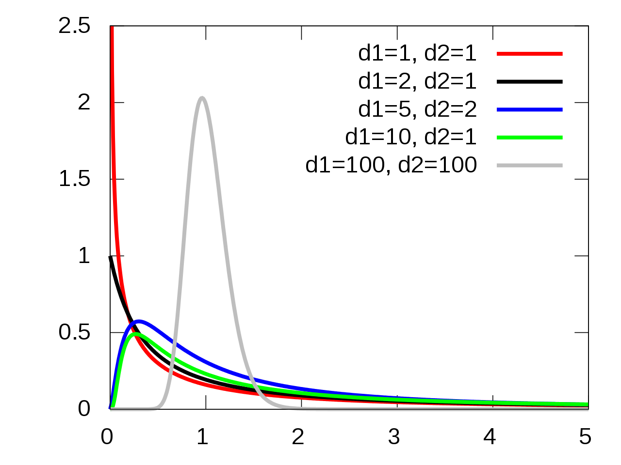
11.3.4 F-Distribution
Under the the following assumptions:
- The null hypothesis is true, i.e., all groups have equivalent means,
- The groups are indendent and normally distributed,
- The groups all have equivalent variances,
the test statistic \(F_t\) follows an \(F(t-1, N-t)\) distribution.
11.3.5 F-Distribution Visualization
11.4 How is this a “Linear Model”
11.4.1 Means Model
Means Model:
\(\begin{aligned} y &= \mu_i + \epsilon \end{aligned}\)
Which leads to the hypotheses in ANOVA:
\(H_0: \mu_{1} = \dots = \mu_{t}\)
\(H_1\): The means are not all equal.
11.4.2 Effects Model
Effects Model:
\(\begin{aligned} y &= \mu + \tau_i + \epsilon \end{aligned}\)
The \(\tau_i\)’s are the shift parameters that cause the groups to differ.
Which leads to an equivalent set of hypotheses:
\(H_0: \tau_{1} = \dots = \tau_{t} = 0\)
\(H_1: \text{Not } H_0\)
11.5 OASIS MRIs
Variables in OASIS data
- Group: whether subject is demented, nondemented, or converted.
- Visit: (Not relevant) which visit number of the MRI
- Gender: M or F
- MR Delay: (Not relevant) time between each successive MRI. First MRIs
- Hand: Handedness of subject. All patients were R (right-handed)
- Age: Age in years
- Educ: Years of education
- SES: Socioeconomic status 1 - 5, low to high SES (arbitrary cutoffs most likely)
- MMSE: Mini Mental State Examination
- CDR: Clinical Dementia Rating, 0 - 2. 0 is non-dementia, CDR > 0 is severity of dementia.
- eTIV: Estimated Total Intracranial Volume (milliliters?)
- nWBV: Normalized Whole Brain Volume; Brain volume is normalized by intercranial volume to put subjects of different sizes and gender on the same scale. To my best knowledge…
- ASF: Atlas Scaling Factor; I tried investigating this but that’s some rabbit hole that is very deep apparently. It has something to do with the normalization I think.
Unlike before, we’re going to compare all three patient groups in the OASIS data: Demented, Nondemented, and Converted.|
Converted patients are those that entered the study that were no diagnosed with dementia, and then by the time the study ended they had been diagnosed with dementia.
The objective is to assess the Normalized Whole Brain Volume nWBV of the different groups and see if the mean nWBV differs.
oasis <- read_csv(here::here("datasets",'oasis.csv'))11.5.1 Examining the data
Let’s look at the nWBVs overall.
nWBVmean <- mean(oasis$nWBV)

### geom_density() produces a "smoothed" histogram.
### if you wanted a histogram, you could use geom_histogram()


ggplot(oasis, aes(x = nWBV)) +
  geom_density(fill = "lavender") +
  geom_vline(xintercept = nWBVmean)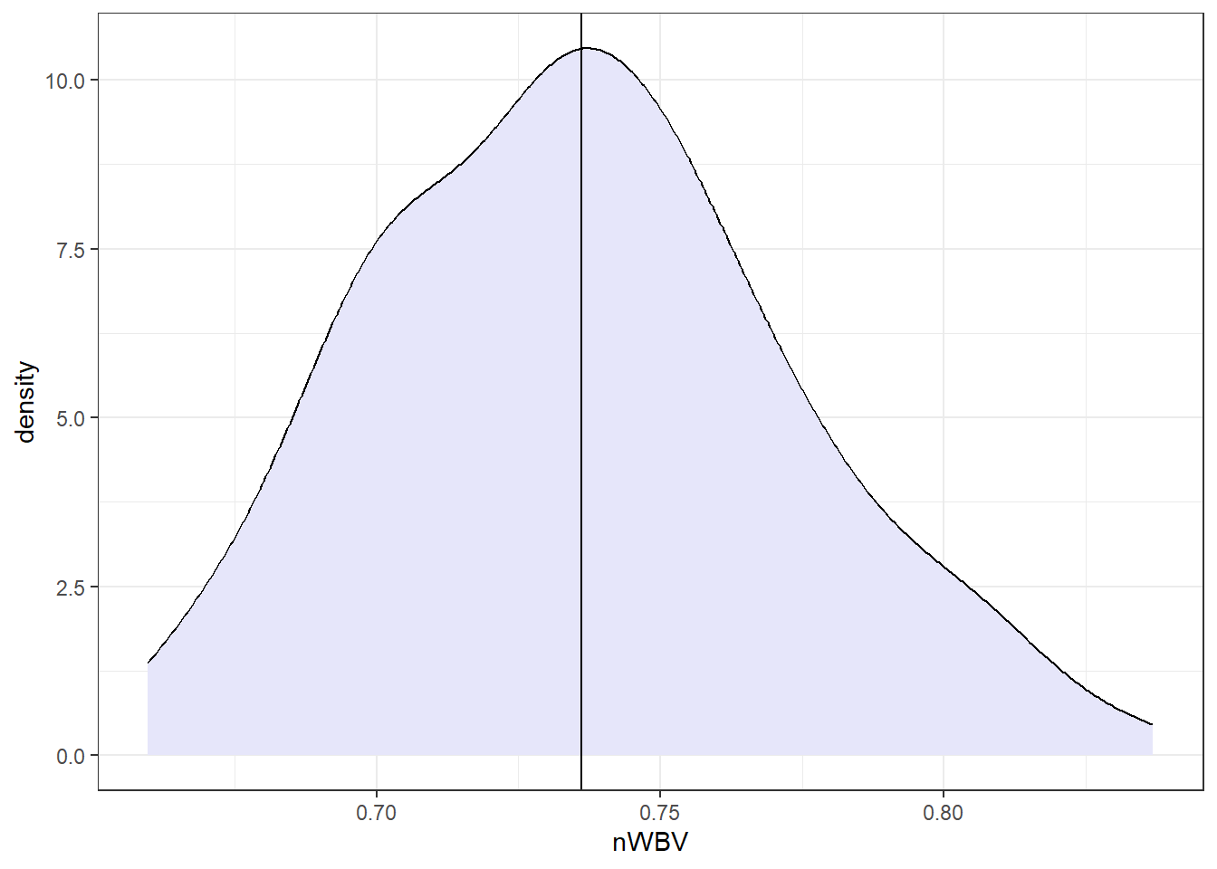
Now let’s look at the grouped data.
# Get group means
## You can ignore this...
ybars <- aggregate(x = nWBV ~ Group, data = oasis,
                   FUN = mean)


ggplot(oasis, aes(x = nWBV, color = Group,
                  fill = Group)) +
  geom_density(alpha = 0.1) +
  geom_vline(data = ybars, aes(xintercept = nWBV,
                               color = Group))
### When comparing groups, a standard way is to use boxplots.
ggplot(oasis, aes(y = nWBV, color = Group,
                  x = Group)) +
  geom_boxplot()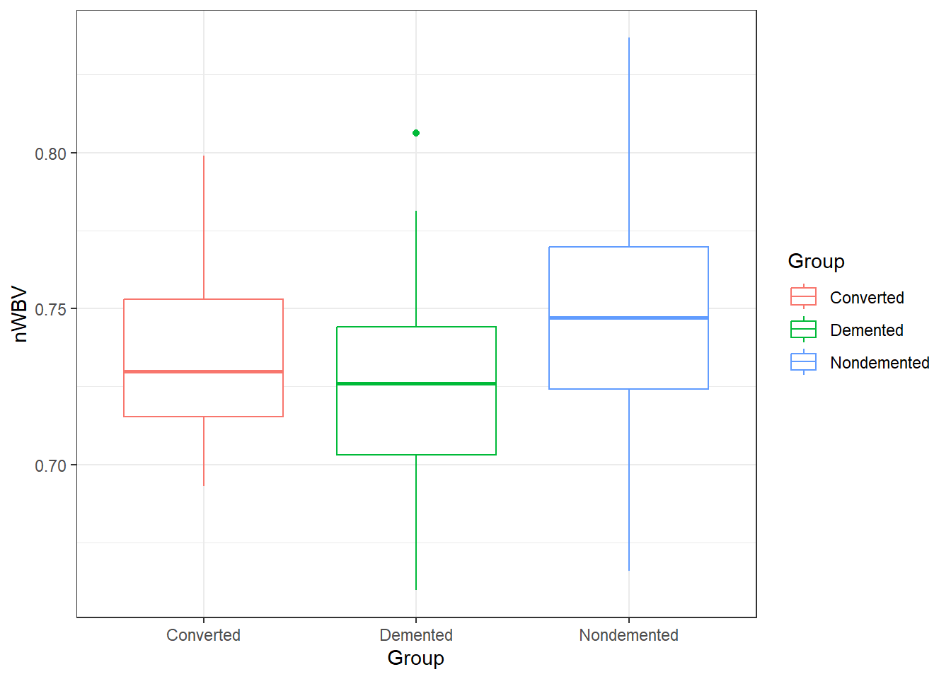
11.5.2 ANOVA in R: its lm() again
There are a few ways to do ANOVA in R. The approach that is most adaptable is to use the lm() function.
lm(formula = y ~ x, data)
So we create a linear model with nWBV as y and Group as x.
fit.lm <- lm(nWBV ~ Group, data = oasis)In general, on lm objects we use the summary() function.
summary(fit.lm)
Call:
lm(formula = nWBV ~ Group, data = oasis)

Residuals:
      Min        1Q    Median        3Q       Max
-0.080200 -0.022459  0.000674  0.023080  0.090780

Coefficients:
                  Estimate Std. Error t value Pr(>|t|)
(Intercept)       0.737860   0.009421  78.317   <2e-16 ***
GroupDemented    -0.013503   0.010401  -1.298    0.196
GroupNondemented  0.008202   0.010297   0.797    0.427
---
Signif. codes:  0 '***' 0.001 '**' 0.01 '*' 0.05 '.' 0.1 ' ' 1

Residual standard error: 0.03525 on 147 degrees of freedom
Multiple R-squared:  0.0806,    Adjusted R-squared:  0.06809
F-statistic: 6.443 on 2 and 147 DF,  p-value: 0.002078
This technically contains all the information we need. Specifically look at the bottom of the summary where there is information on the F-statistic, degrees of freedom and p-value.
To get this information displayed in a more traditional format for an ANOVA, use theanova() function on an lm object.
anova(fit.lm)Analysis of Variance Table
Response: nWBV
Df Sum Sq Mean Sq F value Pr(>F)
Group 2 0.016014 0.0080069 6.4431 0.002078 **
Residuals 147 0.182677 0.0012427
---
Signif. codes: 0 '***' 0.001 '**' 0.01 '*' 0.05 '.' 0.1 ' ' 111.5.3 Alternative: aov()
An alternative is to use the aov() function in the same way:
fit.aov <- aov(nWBV ~ Group, data = oasis)For an aov object, just use the summary() function to get results in a similar manner.
summary(fit.aov) Df Sum Sq Mean Sq F value Pr(>F)
Group 2 0.01601 0.008007 6.443 0.00208 **
Residuals 147 0.18268 0.001243
---
Signif. codes: 0 '***' 0.001 '**' 0.01 '*' 0.05 '.' 0.1 ' ' 1In any of these cases, we have very strong discrepancy with null model (i.e., all means are equal) for a different mean nWBV between the different groups of patients.
11.5.4 Statistical Versus Practical Significance
Let’s look back at the nWBVs split by group:
ggplot(oasis, aes(x = nWBV, color = Group,
                  fill = Group)) +
  geom_density(alpha = 0.10) +
  geom_vline(data = ybars, aes(xintercept = nWBV,
                               color = Group))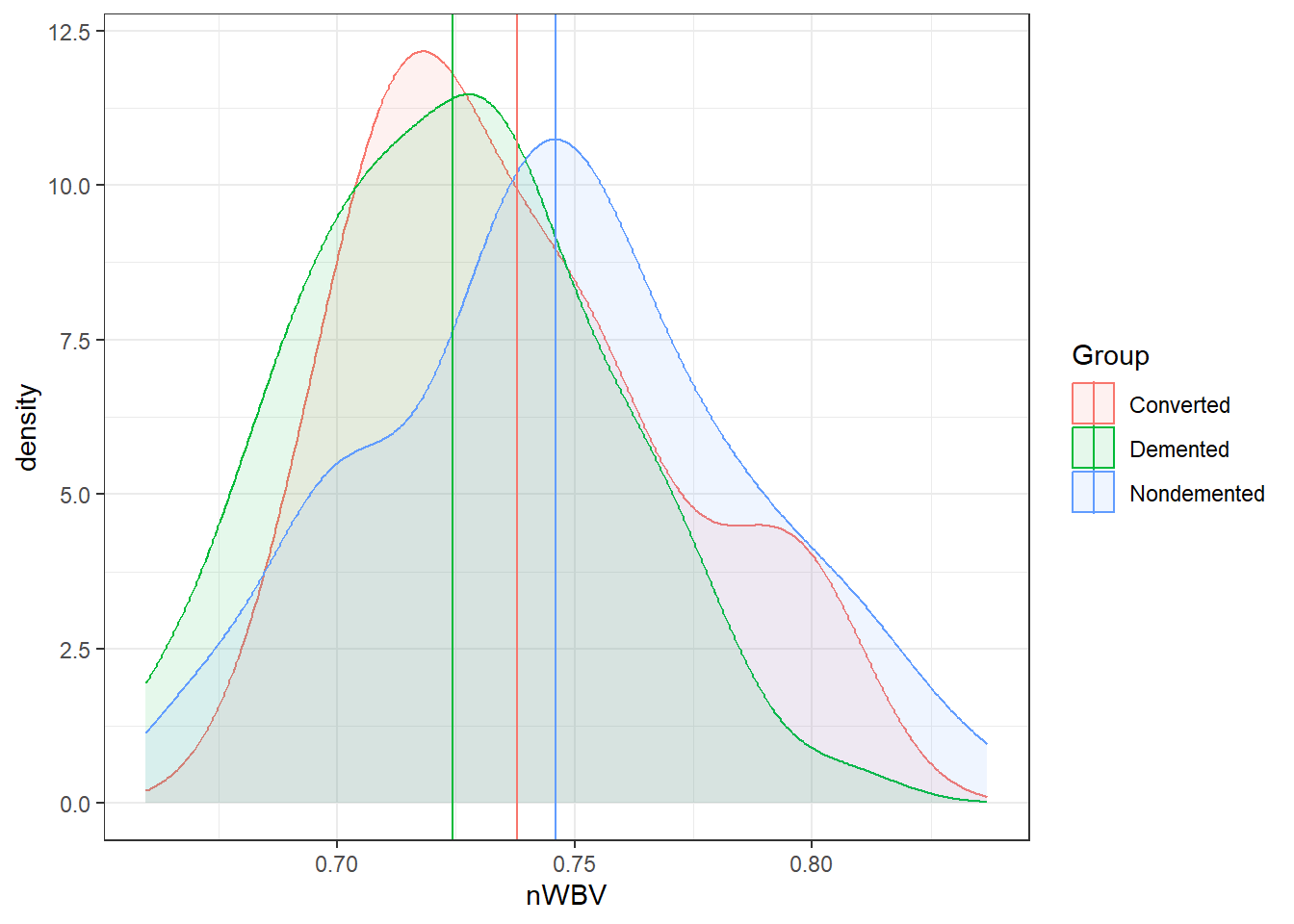
And here are the means of each group.
# This is some tidyverse magic.

oasis %>%
  group_by(Group) %>%
  summarise(mean = mean(nWBV))
# A tibble: 3 × 2
Group mean
<chr> <dbl>
1 Converted 0.738
2 Demented 0.724
3 Nondemented 0.746# Or using the model using modelbased
library(modelbased)
fit.aov %>%
estimate_means()Estimated Marginal Means
Group | Mean | SE | 95% CI
--------------------------------------------
Nondemented | 0.75 | 4.15e-03 | [0.74, 0.75]
Demented | 0.72 | 4.41e-03 | [0.72, 0.73]
Converted | 0.74 | 9.42e-03 | [0.72, 0.76]
Marginal means estimated at GroupAmong the groups, the biggest difference in means between the demented and non-demented group is about 0.02.
Is that a big difference?
- Statistically, it is with \(p = .0021\).
- On a relative scale it is about a 3% difference.
- Is this a practical difference, i.e., does it matter?
- That would be very dependent on the field, the research question, the researcher, the impacts, and so on…
- What is an important difference is a specific matter that should be discussed and defined.