# Here are the libraries I used
library(tidyverse)
library(knitr)
library(readr)
library(ggpubr)5 Inference on the Regression Line
Here are some code chunks that setup this document.
# This changes the default theme of ggplot
old.theme <- theme_get()
theme_set(theme_bw())
# Fun fact. If you put the dataset in the same folder as the Rmd/qmd file you are
# working in. Then you only need the filename to load it. Not the whole file
# path on your computer.
#
# I prefer to use the here package to resolve local path issues
heart <- readr::read_csv(
here::here("datasets","Heart.csv")
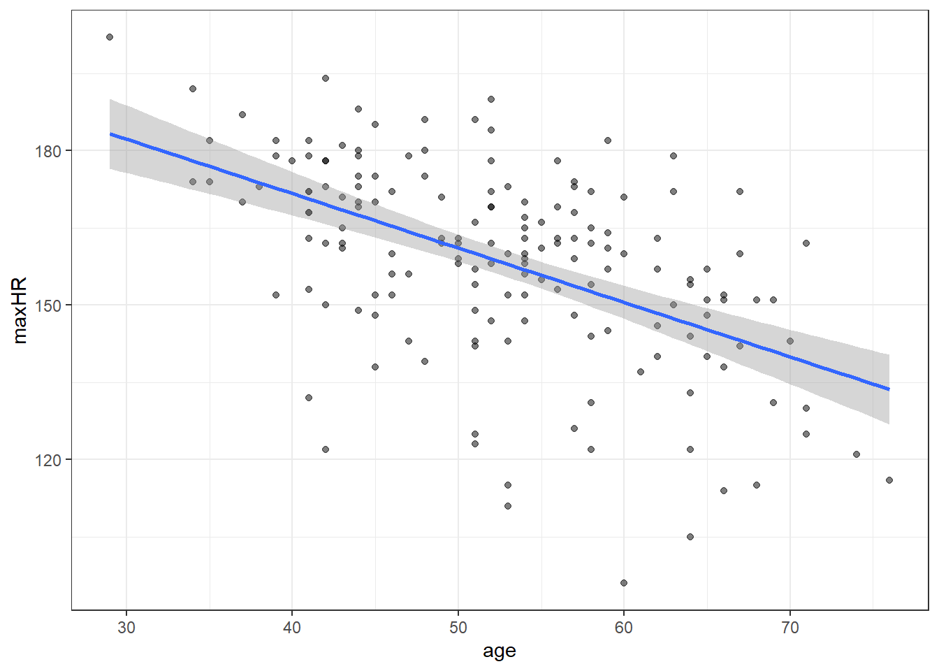
)ggplot(heart, aes(x = age, y = maxHR, color = disease)) +
geom_point() +
geom_smooth(method = "lm", se = FALSE) +
facet_wrap(~disease) +
stat_cor()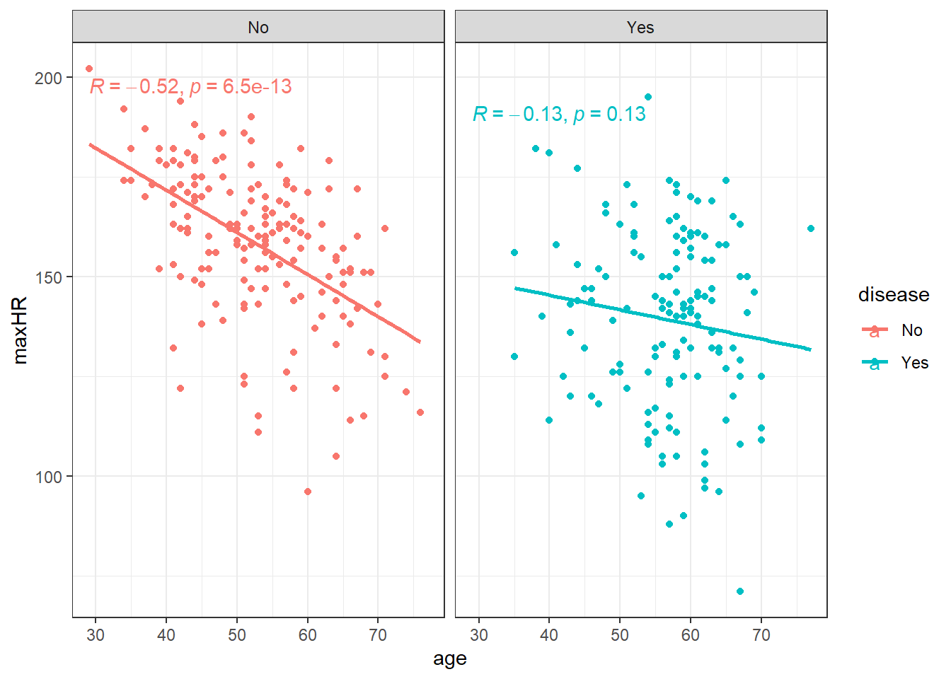
We can filter() the data and only examine individuals without heart disease since the relation doesn’t appear viable in those with heart disease.
noDisease <- filter(heart, disease == "No")ggplot(noDisease, aes(x = age, y = maxHR)) +
geom_point() +
geom_smooth(method = "lm", se = FALSE)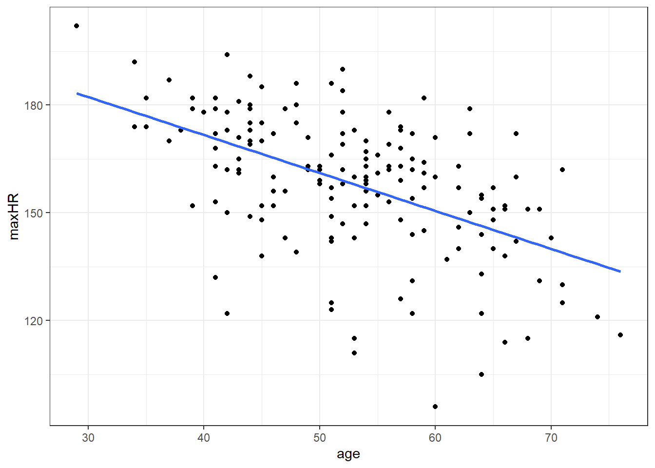
Anyway, there’s a line let’s see what the equation for it is.
# nD is short for no Disease
nD.lm <- lm(maxHR ~ age, noDisease)

nD.lm.sum <- summary(nD.lm)

nD.lm.sum
Call:
lm(formula = maxHR ~ age, data = noDisease)

Residuals:
    Min      1Q  Median      3Q     Max
-54.545  -7.782   2.524  10.004  31.624

Coefficients:
            Estimate Std. Error t value Pr(>|t|)
(Intercept) 213.9282     7.2204  29.628  < 2e-16 ***
age          -1.0564     0.1351  -7.818 6.47e-13 ***
---
Signif. codes:  0 '***' 0.001 '**' 0.01 '*' 0.05 '.' 0.1 ' ' 1

Residual standard error: 16.41 on 162 degrees of freedom
Multiple R-squared:  0.2739,    Adjusted R-squared:  0.2694
F-statistic: 61.12 on 1 and 162 DF,  p-value: 6.469e-13
So the equation to our line would be:
\(\widehat maxHR = 213.9 - 1.06 \cdot age\)
5.0.0.1 Confidence Intervals for Coefficients
confint(nD.lm, level = 0.99) 0.5 % 99.5 %
(Intercept) 195.108145 232.7482574
age -1.408595 -0.7041663
5.1 Uncertainty in the Model
\[y = \beta_0 + \beta_1x + \epsilon_{error}\]
\[\epsilon \sim N(\theta, \sigma_\epsilon)\]
The \(\epsilon\) representing the inherent variability we would expect from individual observations.
5.2 Partitioning Variability
At this point, we will be examining data for those without heart disease only, unless mentioned otherwise.
\[\hat y = \widehat \mu_{y|x} = \widehat\beta_0 + \widehat\beta_1 x\]
5.2.1 Sums of Squares
\[SSTO = \Sigma_{i=1}^n (y_i - \bar y)^2\]
\[ s^2_y = \frac{SSTO}{n-1} \]
This variability in the variable can be broken up into two pieces:
- The Sum of Squares of Regression \(SSR\).
\[SSR = \Sigma(\hat y - \bar y)^2\]
- The Sum of Squared Error \(SSE\).
\(SSE = \Sigma (y_i - \hat y_i)^2\)
The two sums of squares combined are the total variability \(SSTO\).
\(SSTO = SSR + SSE\)
5.2.2 Coefficient of Determination \(R^2\)
\(R^2 = \frac{SSR}{SSTO} = \frac{Explained}{Total}\)
which is the ratio of how much of the total variability in our data that is “explained” by our model.
Often the form of \(R^2\) is written as
\(R^2 = 1- \frac{SSE}{SSTO}\)
5.2.2.1 Interpreting \(R^2\)
“The regression model is accounting for <\(R^2\cdot 100\)>% of the variability in <the response variable.”
nD.lm.sum
Call:
lm(formula = maxHR ~ age, data = noDisease)

Residuals:
    Min      1Q  Median      3Q     Max
-54.545  -7.782   2.524  10.004  31.624

Coefficients:
            Estimate Std. Error t value Pr(>|t|)
(Intercept) 213.9282     7.2204  29.628  < 2e-16 ***
age          -1.0564     0.1351  -7.818 6.47e-13 ***
---
Signif. codes:  0 '***' 0.001 '**' 0.01 '*' 0.05 '.' 0.1 ' ' 1

Residual standard error: 16.41 on 162 degrees of freedom
Multiple R-squared:  0.2739,    Adjusted R-squared:  0.2694
F-statistic: 61.12 on 1 and 162 DF,  p-value: 6.469e-13
Regardless of how we get it, an interpretation of the model would be “using a linear model, age accounts for approximately 27% of the variability in maximum heart rate”.
5.3 Analysis of Variance (ANOVA) in Regression
In simple linear regression we discussed the hypothesis test for the slope (and intercept).
\[H_0: \beta_1 = 0\]
- Essentially, null hypothesis posits that x variable is useless as predictor of y
\[H_1: \beta_1 \neq 0\]
In essence we are testing to see if the \(x\) variable is a worthwhile predictor.
This test was done via the test statistic \[t = \frac{\hat \beta_1}{SE_{\hat \beta_1}}.\]
The \(t\) distribution with \(n-2\) degrees of freedom is used to compute the \(p\)-value for this hypothesis test.
5.3.1 Degrees of Freedom
\(SSR\) has 1 degree of freedom.
\(SSE\) has \(n-2\) degrees of freedom.
Overall, \(SSTO\) has \(n-1\) degrees of freedom.
5.3.2 Mean Squares and the Test Statistic
However, in regression analysis, we are mainly interested in the mean square of regression \(MSR\) and mean squared error.
A mean square is the sum of square divided by its degrees of freedom.
- \(MSR = \frac{SSR}{1}\)
- \(MSE = SSE \div (n-2)\)
We take their ratio, which is our new test statistic.
\(F_t = \frac{MSR}{MSE} = \frac{SSR}{1} \div \frac{SSE}{n-2}\)
F-test under \(H_0\)
\[ H_0 \rightarrow F_t \sim F(1,n-2) \]
5.3.3 F-Distribution
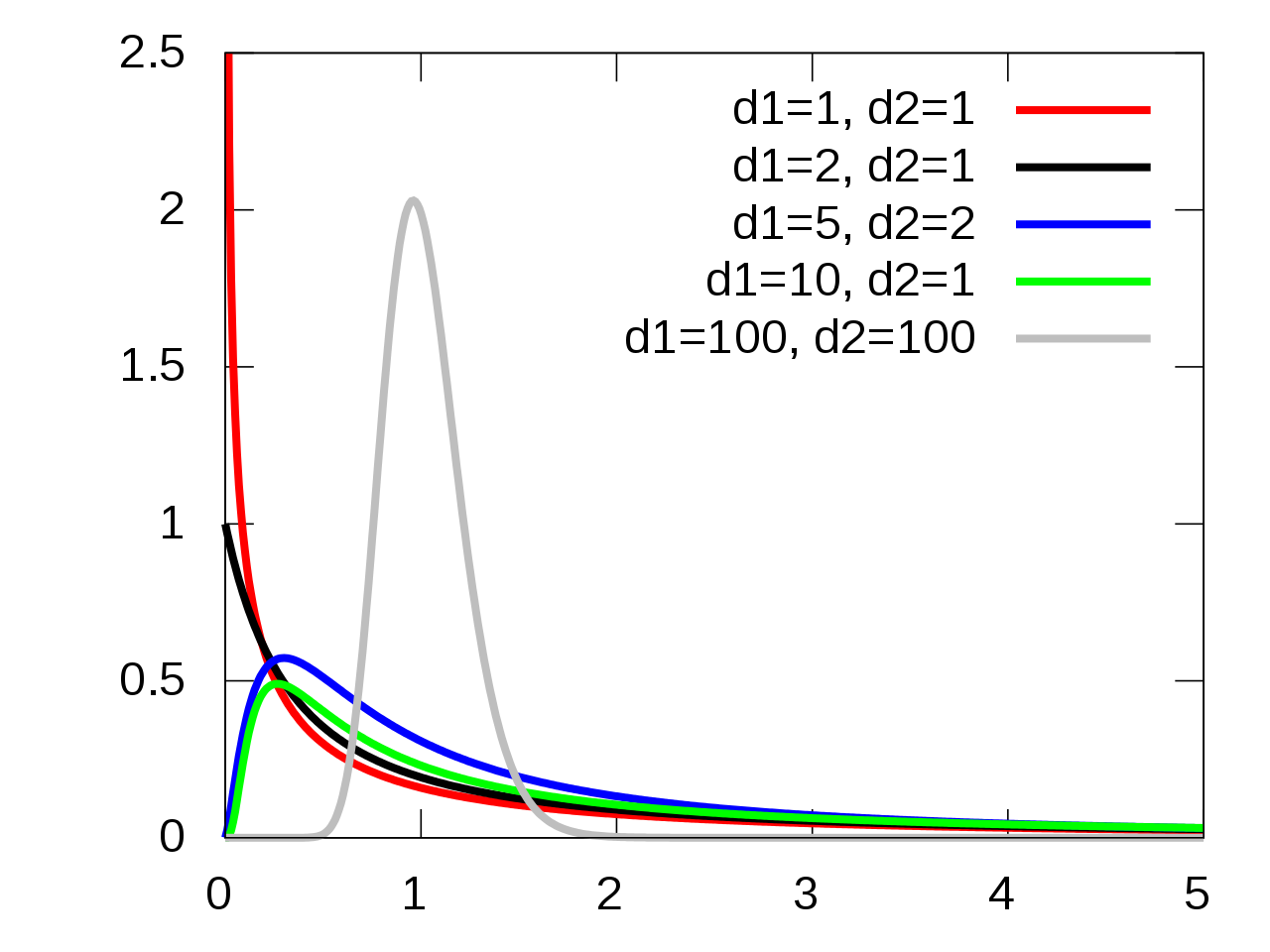
The \(p\)-value is the probability of a random value from an \(F(1, n-2)\) distribution exceeding the test statistic: \(p = P\left(F(1, n-2) > F_t\right)\).
library(ggdist)
library(distributional)

dist_df = data.frame(
  d = dist_f(1,18)
)

dist_df %>%
  ggplot(aes(xdist = d)) +
  stat_slab(color = "grey", expand = TRUE,
            aes(fill = after_stat(level)),
            .width = c(.95,1))+
  stat_spike(at = function(x) hdci(x, .width = .975),
             linetype = "dashed")+
  # need shared thickness scale so that stat_slab and geom_spike line up
  scale_thickness_shared() +
  theme_void() +
    scale_fill_brewer(na.value = "gray95") +
  labs(fill = "Rejection Region on F-distribution",
       caption = "F distribution with 1 and 18 degrees of freedom") +
  theme(legend.position = "none")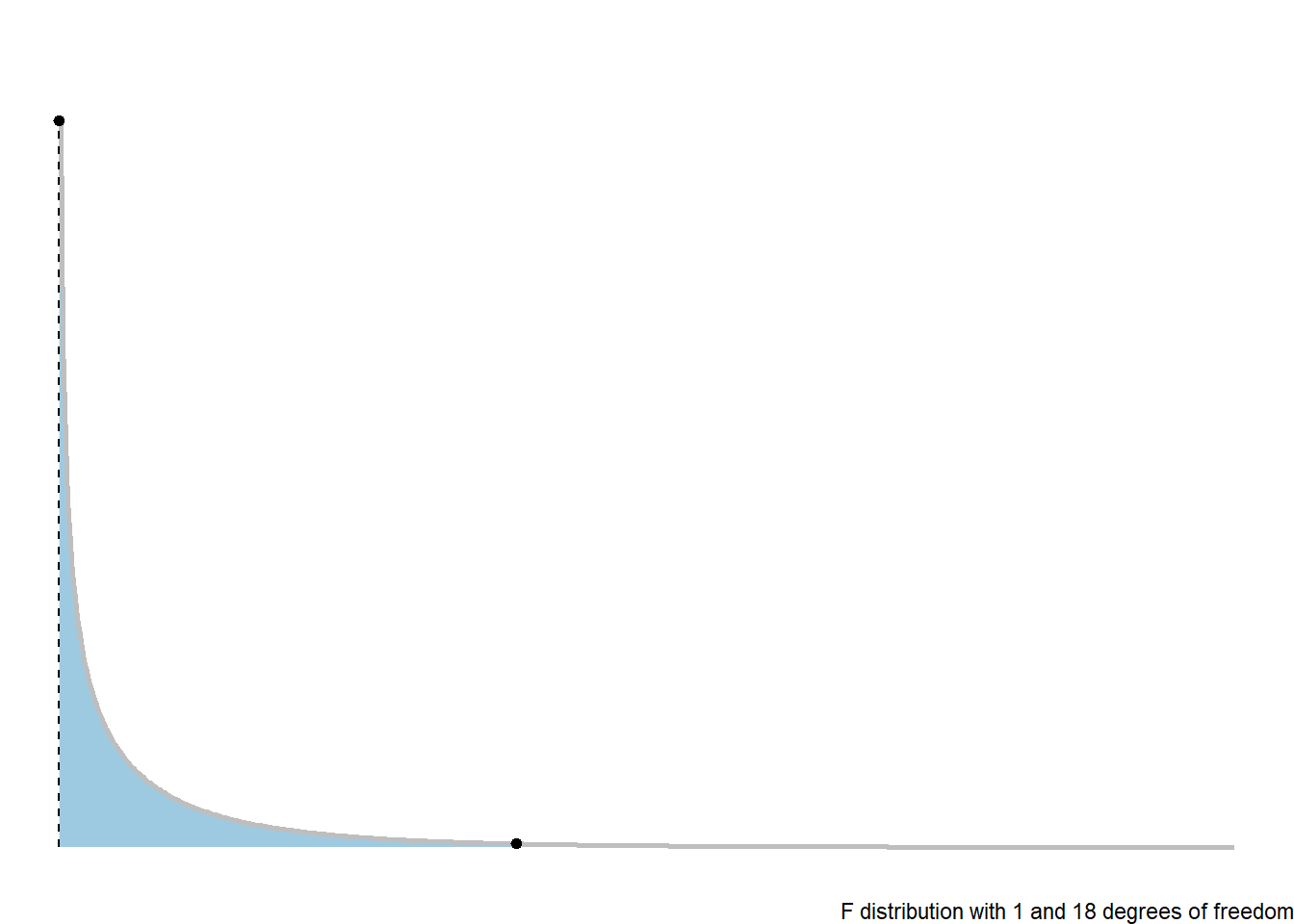
5.3.4 ANOVA Table
We would in general summarise a Analysis of Variance based hypothesis test with the following ANOVA table.
| Source of Variability | Sum of Squares | df | MS | F | p-value |
|---|---|---|---|---|---|
| Regression/Model | \(SSR\) | \(1\) | \(MSR = SSR/1\) | \(F_t = MSR/MSE\) | \(p\) |
| Error | \(SSE\) | \(n-2\) | \(SSE/(n-2)\) | ||
| Total | \(SSTO\) | \(n-1\) |
5.3.5 Regression ANOVA in R
The ANOVA hypothesis test information is shown in the last row of the summary of an lm.
nD.lm.sum
Call:
lm(formula = maxHR ~ age, data = noDisease)

Residuals:
    Min      1Q  Median      3Q     Max
-54.545  -7.782   2.524  10.004  31.624

Coefficients:
            Estimate Std. Error t value Pr(>|t|)
(Intercept) 213.9282     7.2204  29.628  < 2e-16 ***
age          -1.0564     0.1351  -7.818 6.47e-13 ***
---
Signif. codes:  0 '***' 0.001 '**' 0.01 '*' 0.05 '.' 0.1 ' ' 1

Residual standard error: 16.41 on 162 degrees of freedom
Multiple R-squared:  0.2739,    Adjusted R-squared:  0.2694
F-statistic: 61.12 on 1 and 162 DF, p-value: 6.469e-13anova(nD.lm)Analysis of Variance Table
Response: maxHR
Df Sum Sq Mean Sq F value Pr(>F)
age 1 16458 16457.7 61.115 6.469e-13 ***
Residuals 162 43625 269.3
---
Signif. codes: 0 '***' 0.001 '**' 0.01 '*' 0.05 '.' 0.1 ' ' 15.4 Model Error: \(\sigma_\epsilon\)
This is the linear model for each value \(y\) value in a random sample:
\(y_i = \beta_0 + \beta_1 x_i + \epsilon_i\)
Where of particular note, we have
variability:
\[\epsilon_i \sim N(0, \sigma_\epsilon)\]
\[\hat \sigma_\epsilon= \sqrt{MSE}\]
5.4.1 Standard Error of \(\hat \beta_1\) and \(\widehat \beta_0\)
\[SE_{\beta_0}= \hat \sigma_{\epsilon}\sqrt{\dfrac{1}{n} + \dfrac{\overline x^2}{\sum(x_i - \overline x)^2}}\]
\[SE_{\beta_1} = \hat \sigma_{\epsilon}\sqrt{\dfrac{1}{\sum(x_i - \overline x)^2}}\]
5.4.2 Standard Error for the Line
We use the equation
\[\hat y= \hat \mu_{y|x} = \beta_0 + \beta_1 x\]
How uncertain are we estimating the mean, or making predictions?
5.4.2.1 Estimated Conditional Mean
When estimating \(\mu_{y|x}\) at a given value of \(x\), the standard error is:
\[SE_{\hat \mu_{y|x}} = \hat \sigma_{\epsilon} \sqrt{\dfrac{1}{n} + \dfrac{(x-\overline x)^2}{\sum(x_i - \overline x)^2}}\]
This is the counterpart to what you did in your introductory course when just estimating the mean of \(y\) (\(\mu\)) without considering an \(x\) variable.
\[SE_{\bar y }= \frac{s}{\sqrt{n}}\]
5.4.2.2 Standard Error of Predictions
\[SE_{pred} = \hat \sigma_{\epsilon} \sqrt{1 + \dfrac{1}{n} + \dfrac{(x-\overline x)^2}{\sum(x_i - \overline x)^2}}\]
5.4.3 Confidence Intervals for the Mean
We can use our data and compute an estimated value for the line:
\[\hat \mu_{y|x} = \beta_0 + \beta_1 x\]
We can create confidence intervals for this estimate using the \(t\)-distributiuon with \(n-2\) degrees of freedom.
\[\hat \mu_{y|x} + t_{\alpha/2,df} \cdot SE_{\hat \mu_{y|x}}= \hat \mu_{y|x} \pm t_{\alpha/2, n-2} \hat \sigma_{\epsilon} \sqrt{\dfrac{1}{n} + \dfrac{(x-\overline x)^2}{\sum(x_i - \overline x)^2}}\]
This interval tells us that we can be \((1-\alpha)100\%\) confident that the true line at a given point \(x\) is between the lower and upper bound.
5.4.4 Prediction Intervals for Future Observations
In a similar manner, we can create confidence intervals that will let us be \((1-\alpha)100\%\) confident that a future observation will be between
\[\widehat y \pm t_{\alpha/2, n-2} SE_{pred} = \hat y \pm t_{\alpha/2, n-2} \hat \sigma_{\epsilon} \sqrt{1 + \dfrac{1}{n} + \dfrac{(x-\overline x)^2}{\sum(x_i - \overline x)^2}}\]
5.4.5 Getting Confidence and Prediction Intervals in R
For confidence and prediction intervals, we can use the predict(). The arguments we need to define are interval and level.
intervalcan be set to “none”, “confidence”, and “prediction” for no interval, a confidence interval for the mean, and a future observation prediction interval, respectivelylevelis simply the confidence level of your interval. The default is 0.95.
# need the data for predictions

predData <- data.frame(age = c(20, 30, 40, 50, 60, 70, 80))

confIntervals <- predict(nD.lm, newdata = predData, interval = "confidence", level = 0.99)
predIntervals <- predict(nD.lm, newdata = predData, interval = "prediction", level = 0.99)
Confidence Intervals:
confIntervals fit lwr upr
1 192.8006 180.8474 204.7537
2 182.2368 173.6092 190.8644
3 171.6730 166.1228 177.2232
4 161.1092 157.6473 164.5711
5 150.5454 146.3056 154.7852
6 139.9816 132.9975 146.9657
7 129.4178 119.2006 139.6349Prediction Intervals:
predIntervals fit lwr upr
1 192.8006 148.38873 237.2125
2 182.2368 138.60227 225.8713
3 171.6730 128.54132 214.8046
4 161.1092 118.19624 204.0221
5 150.5454 107.56269 193.5281
6 139.9816 96.64206 183.3211
7 129.4178 85.44134 173.39425.4.6 Graph of Confidence Intervals and Prediction Intervals
# without giving predict() new data,
# you get predictions for ALL points in the data
predictions <- predict(nD.lm,
                       interval = "prediction",
                       level = 0.99)

# combin prediction intervals with dataset
allData <- cbind(noDisease, predictions)

# graph
 #define x and y axis variables
ggplot(allData, aes(x = age, y = maxHR)) +
  geom_point() + #add scatterplot points
  stat_smooth(method = lm, level = 0.99) + #confidence bands
  geom_line(aes(y = lwr), col = "red",
            linetype = "dashed") + #lwr pred interval
  geom_line(aes(y = upr), col = "red",
            linetype = "dashed") #upr pred interval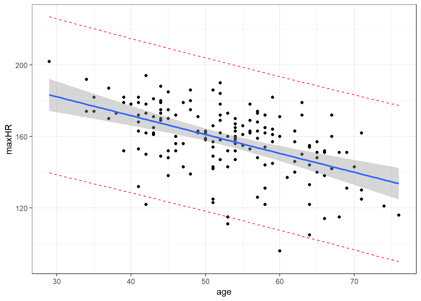
Blue is estimated line, gray is possibilities for true line, and red is a range possible future observations.
5.4.7 Important Note: Confidence Levels and Their Reliability.
The confidence level for a confidence/prediction interval only applies to that individual interval.
5.5 Working-Hotelling Confidence:
The calculation of confidence and prediction bands if fairly simple. You just have to replace the critical \(t\) value used to create the confidence and prediction interval. This replacement is based off of a modification of values from the F-Distribution.
This value will be referred to is as \(W_\alpha\). It requires a value from the \(F\) distribution with 2 degrees of freedom for the numerator, and \(n - 2\) for the denominator. This value on the \(F\) distribution is such that it has a left-tail area/probability of \(1-\alpha\).
\[ W_\alpha = \sqrt{2\cdot F(1-\alpha, 2, n-2)}\]
5.5.1 Working-Hotelling Confidence Bands
To compute the confidence bands, the formula is:
\[\widehat y \pm t_{\alpha/2, n-2} \cdot SE_{pred} = \hat y \pm W_\alpha \space \sqrt{1 + \dfrac{1}{n} + \dfrac{(x-\overline x)^2}{\sum(x_i - \overline x)^2}}\]
5.5.2 Working-Hotelling Prediction Bands Bands
Similarly for the prediction intervals.
\[\widehat y \pm t_{\alpha/2, n-2} SE_{pred} = \hat y \pm W_\alpha \hat \sigma_{\epsilon} \sqrt{1 + \dfrac{1}{n} + \dfrac{(x-\overline x)^2}{\sum(x_i - \overline x)^2}}\]
5.5.3 Getting These in R
Apparently I need to make my own R functions for this.
working_hotelling_intervals <- function(x, y) {
  y <- as.matrix(y)
  x <- as.matrix(x)
  n <- length(y)

  # Get the fitted values of the linear model
  fit <- lm(y ~ x)
  fit <- fit$fitted.values

  # Find standard error as defined above
  se <- sqrt(sum((y - fit)^2) / (n - 2)) *
    sqrt(1 / n + (x - mean(x))^2 /
           sum((x - mean(x))^2))

  # Calculate B and W statistics for both procedures.
  W <- sqrt(2 * qf(p = 0.95, df1 = 2, df2 = n - 2))
  B <- 1-qt(.95/(2 * 3), n - 1)

  # Compute the simultaneous confidence intervals

  # Working-Hotelling
  wh.upper <- fit + W * se
  wh.lower <- fit - W * se

  xy <- data.frame(cbind(x,y))

  # Plot the Working-Hotelling intervals
  wh <- ggplot(xy, aes(x=x, y=y)) +
    geom_point(size=2.5) +
    geom_line(aes(y=fit, x=x), size=1) +
    geom_line(aes(x=x, y=wh.upper),
              colour='blue', linetype='dashed') +
    geom_line(aes(x=x, wh.lower),
              colour='blue', linetype='dashed') +
    labs(title='Working-Hotelling')


  return(wh)
}

working_hotelling_intervals(x = noDisease$age, y = noDisease$maxHR)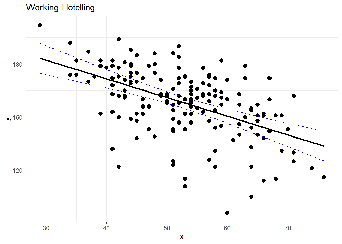
# compare with ggplot
#
ggplot(noDisease,
       aes(x=age,
           y=maxHR)) +
  geom_point(alpha = .5) +
  geom_smooth(method = "lm",
              formula = y~x,
              se = TRUE)