1 Review of Introductory Inference

1.1 Review: Inference

There is some expectation of knowledge that you should know from your previous statistics course.

Key concepts you are expected to have knowledge of:

Populations and samples
Probability
Random variables
Probability distributions
- probability density functions
- cumulative distribution functions
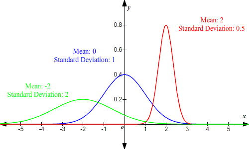
- Normal distribution
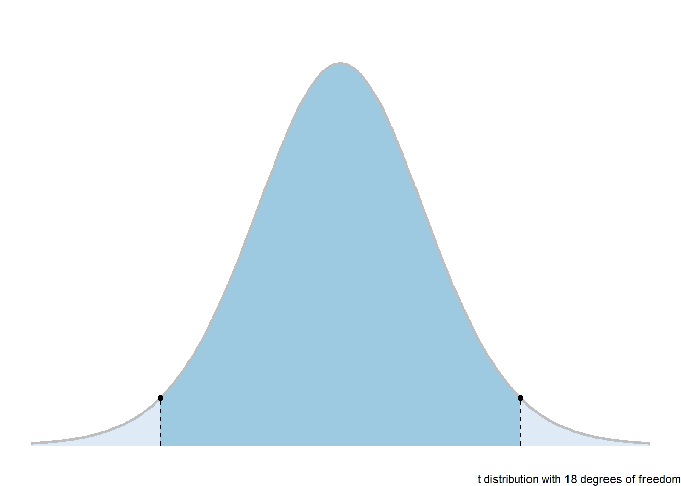
- \(t\) distribution
- \(F\) distribution
Sampling distributions
Confidence intervals and hypothesis tests
- one-sample mean
- two-sample means

There will be a brief review of some of the more topics and a set of materials will be linked to at the end of this appendix.

1.2 General Idea of Inference

We will cover some of the topics you should know from a previous introductory course in statistics. There is a general procedure that we can conceptualize.

There is a general target population we are interested in in some way.
We have certain questions we want to ask about this population.
We figure out what can we quantify from the population and how those quantfications may answer our questions.
We collect our data/measurements from the population.
- Sometimes (maybe often) the way we collect data changes the exact nature of the population we are interested in.
We perform statistical analyses/inference on the population to see how the data answers our questions.
We communicate our findings in some way… Typically.

1.2.1 Populations and Parameters: Means and Standard Deviations

If I have some population \(Y\):

\[ \bar Y \rightarrow Random \space Variable \rightarrow Population \]

\(\mu\): mean
\(\sigma\): standard deviation

1.2.2 Estimating The Mean and Standard Deviation

We estimate the mean of a population by taking a sample. We assume simple random samples; you might want to look up what the means if you forgot.

The estimate of a population mean \(mu\) is the sample mean which is typically denoted by \(\bar y\).

\[ \bar y = \frac{\Sigma y_i}{n} \rightarrow estimate \space \mu \]

The estimate of the population standard deviation \(\sigma\) is the sample standard deviation, denoted by \(s\).

\[ \hat \sigma = s = \sqrt{\frac{\Sigma(y_i - \bar y )^2}{n-1}} \]

We refer to these statistics as point estimates. This term is used to emphasize the fact that we have some fixed number when we do the calculation.

1.3 Central Limit Theorem, Standard Errors, and Uncertainty

1.3.1 Standard Error

The standard measure of reliability for \(\bar y\) is the standard error.

\[ \sigma_{\bar y} = \frac{\sigma}{\sqrt{n}} \]

1.3.1.1 Estimated SE

\[ SE_{\bar y}= \frac{s}{\sqrt{n}} \]

This is our measurement of relative uncertainty of the sample mean.

1.3.2 Central Limit Theorem

The standard error is an important part of the Central Limit Theorem (CLT). The barebones of the CLT is:

\[ \bar y \sim N(\mu, \frac{\sigma}{\sqrt{n}} ) \]

SE: \(\frac{s}{\sqrt{n}}\)
t-distribution

The CLT allows us to, under certain assumptions, figure a range of likely values for the true mean \(\mu\). These assumptions are either:

The population we take the sample from is approximately normally distributed, or
We have a sufficiently large sample size that we can ignore assumption 1. “Sufficiently large” is typically characterized as \(n > 30\), but that rule-of-thumb would depend on the population distribution.

A link to a demonstration is here: https://gallery.shinyapps.io/CLT_mean/

1.4 Confidence Intervals for the Mean

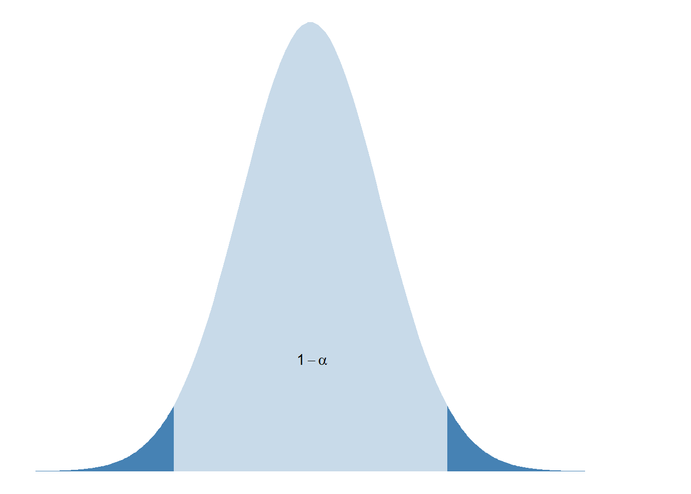
This is the \((1-\alpha)100\%\) confidence interval for \(\mu\).

\[ \bar y \pm t_{\alpha/2, df} \frac{s}{\sqrt{n}} \]

Margin of Error
The confidence level \((1-\alpha) \cdot 100\%\) is the reliability of a computed interval.
\(t_{\alpha/2, df}\) is the value from the \(t\) distribution with a right tail area of \(\alpha/2\) and degrees of freedom \(df = n - 1\). The degrees of freedom formula will change depending on what is being estimated.

1.4.1 General Form for Confidence Intervals

There are many situations where we are estimating some parameter \(\theta\) of a population.

Let \(\hat \theta\) represent the estimate of \(\theta\).

\[ \hat \theta \pm t_{\alpha/2, df} \cdot {SE}_{\hat \theta} \]

1.5 Hypothesies Tests

A hypothesis test is a statistics procedure that is meant to assess the validity that a population parameter \(\theta\) differs from some predefined value \(\theta_0\).

The basic procedure is this:

Hypotheses about \(\theta\)

\(H_0: \space \theta = \theta_0\)
\(H_1: \space \theta \neq \theta_0\)

Collect data and estimate \(\theta\) with \(\hat \theta\)
Test statistic

\[ t_s = \frac{ \hat \theta - \theta_0} { SE_{\hat \theta}} \] 4. p-value \(p = Pr(T_y \ge |t_s|)\)

\(p < \alpha\), if yes then reject \(H_0\)
Remember, \(\alpha\) is the desired type 1 error rate

1.6 Review Videos (courtesy of JB Statistics and Crash Course)

Given that this is material that you are expected to know for this class, I am only putting this here as a reminder, and for you to gauge yourself on how much you remember.

Should you feel that you need a refresher, the website and book of Balka (n.d.) provides a fairly thorough break of any and all the topics you should know about coming into this course from Biostatistics 101.

I’ve provided links to some of the videos relevant to the pre-requisite material.