15 Unbalanced Two-Factor Analysis of Variance

Here are some code chunks that setup this chapter.

# Here are the libraries I used
library(tidyverse) # standard
library(knitr) 

library(readr) # need to read in data
library(ggpubr) # allows for stat_cor in ggplots
library(ggfortify) # Needed for autoplot to work on lm()
library(gridExtra) # allows me to organize the graphs in a grid
library(car) # need for some regression stuff like vif
library(GGally)
library(emmeans)

# This changes the default theme of ggplot
old.theme <- theme_get()
theme_set(theme_bw())

An Unbalanced ANOVA involves data where individual treatments/cells do not have the same number of observations/subjects.

The principals remain the same:

\(y\) is our response variable
We can have various \(x\) variables that we are manipulating.
- In ANOVA context these are called factors.
- We can have more than one factor. (Technically as many as we want, but probably stop at 3!)
- Each factor has a set of levels, i.e. the specific values that are set
- A treatment is the specific combination of the levels of all the factors.
We wish to assess which factors are important in our response variable.
The main diffference with unbalanced data is that the hypothesis tests become a little more obtuse.

15.1 Two way ANOVA Model

This is still the same! It’s just copy pasted from previous section.

There is a means model:

\[y = \mu_{ij} + \epsilon\]

\(\mu_{ij}\) is the mean of treatment \(A_iB_j\).
Epsilon is the error term and it is assumed \(\epsilon \sim N(0, \sigma)\).
- The constant variability assumption is here.

Which in my opinion is not congruent with what we are trying to investigate in Two-Way ANOVA.

We are trying to understand the effect that both factors have on the the response variable.
There may be an interaction between the factors.
- This is when the effect the levels of factor A is not consistent across all levels of factor B, and vice versa.
- For example, the mean of the response variable may increase when going from treatment \(A_1B_1\) to \(A_2B_1\), but the response variable mean decreases when we look at \(A_1B_2\) to \(A_2B_2\).

With this all in mind, the effects model in two-way ANOVA is:

\[y = \mu + \alpha_i + \beta_j + \gamma_{ij} + \epsilon\]

\(\mu\) would be the mean of the response variable without the effects of the factors.
- This can usually be thought of as the mean of a control group.
\(\alpha_i\) can be thought of as the effect that level \(i\) of factor A has on the mean of \(y\).
Likewise, \(\beta_j\) is the effect that level \(j\) of factor B has on the mean of \(y\).
\(\gamma_{ij}\) is the interaction effect, which is the additional effect that the specific combination \(A_i\) and \(B_j\) has on the mean of \(y\).

15.2 Notation and jargon

There’s a lot here. The notation logic is fairly procedural (to a degree that it becomes confusing).

Factors and Treatments

We have factor A with levels \(i = 1,2, \dots, a\) and factor B with levels \(j = 1,2, \dots, b\).

\(A_i\) represents level \(i\) of factor \(A\).
\(B_j\) represents level \(j\) of factor \(B\).
\(A_iB_j\) represents the treatment combination of level \(i\) and level \(j\) of factors A and B respectively.
This is sometimes referred to as “treatment ij”.

Sample Sizes

This is where things get sketchier/more obsuse. We have to account for the fact that each \(A_iB_j\) treatment group may have a different sample size.

\(n_{ij}\) is the number of observations/subjects in treatment \(A_iB_j\).
\(n_{i.}\) represents the total number of observations in \(A_i\). (\(n_{i.} = \sum_{j=1}^bn_{ij}\))
\(n_{.j}\) represents the total number of observations in level \(i\) of factor A. (\(n_{.j} = \sum_{i=1}^a n_{ij}\))
\(n_{..}\) (or sometimes \(N\)) represents the total number of observations overall. (\(n_{..} = \sum_{i=1}^a \sum_{j=1}^b n_{ij}\))

Observations and Sample Means

An individual observation is denoted by \(y_{ijk}\). The subscripts indicate we are looking at observation \(k\) from treatment \(A_iB_j\)

Since there are \(n_{ij}\) observations in each individual treatment treatment, \(k = 1,2, \dots, n_{ij}\).
\(\overline y_{ij.}\) is the mean of the observations in treatment \(A_iB_j\). (\(\overline y_{ij.} =\frac{1}{n_{ij}} \sum_{k=1}^{n_{ij}}y_{ijk}\))
\(\overline y_{i..}\) is the mean of the observations in treatment \(A_i\) across all levels of factor B. (\(\overline y_{i..} = \frac{1}{n_{i.}}\sum_{j=1}^{b}\sum_{k=1}^{n_{ij}}y_{ijk}\))
\(\overline y_{.j.}\) is the mean of the observations in treatment \(B_j\) across all levels of factor A. (\(\overline y_{.j.} = \frac{1}{n_{.j}}\sum_{i=1}^{a}\sum_{k=1}^{n_{ij}}y_{ijk}\))
\(\overline y_{...}\) is the mean of all observations. (\(\overline y_{...} = \frac{1}{n_{..}}\sum_{i=1}^{a}\sum_{j=1}^{b}\sum_{k=1}^{n_{ij}}y_{ijk}\))

15.3 Sums of Squares in Unbalanced Designs

This is where things get tricky in unbalanced designs. We are forgoing formulas at this point because they become somewhat less meaningful.

In order for you to safely perform these hypothesis tests, you have to consider how you are testing them.
If we were to follow the pattern of say multiple regression or one-way ANOVA, we could separate the variability explained by each factor.

\[SSA = \text{Variability Explained by Factor A}\]

SSA would what is used to test \(H_0: \alpha_i = 0\) for all \(i\).

\[SSB = \text{Variability Explained by Factor B}\]

SSB would what is used to test \(H_0: \beta_j = 0\) for all \(j\).

\[SSAB = \text{Variability Explained by interaction between A and B}\]

SSAB would what is used to test \(H_0: \gamma_{ij} = 0\) for all \(i,j\).

However… In unbalanced designs, we no longer have access to these simplified sums of squares and hypothesis tests

There become 3 different mainstream types of ANOVA Hypothesis Tests

15.4 The Forsest of Sums of Squares

There are many ways of framing the sums of squares in unbalanced ANOVA as care must be taken.

The notation here is changing to emphasize that we are looking at fundamentally different things now.

\(SS(A)\) is the amount of variability explained by factor A in a model by itself,
\(SS(B)\) is the amount of variability explained for by factor B in a model by itself.
\(SS(AB)\) is the amount of variability explained for by interaction in a model by itself.
\(SS(A|B)\) is the additional variability explained for by factor A when factor B is in the model
- \(SS(A|B,AB)\) is the additional variability explained for by factor A when factor B and the interaction are in the model.
\(SS(B|A)\) is the additional variability explained for by factor B when factor A is in the model.
- \(SS(B|A,AB)\) is the additional variability explained for by factor A when factor B and the interaction are in the model.
\(SS(AB|A,B)\) is the additional variability explained for by the interaction when factor B and A are in the model.

The sum of squares are now about how much more a factor or interaction can contribute to a model. Not whether it is in the model or not.

15.5 Hypothesis Tests

There are three types of tests that use these sums of squares.

Type I: “Sequential”.
TYpe II: “Marginality” (This is a hill some people choose to die on it seems.)
Type III: “???”

15.5.1 Type I Tests

Type I tests are about sequentially adding terms, starting with the factors then moving up to higher order terms (interaction).

The sequence of hypothesis tests would be the following.

Start with one factor, the test would be:

\(H_0: \mu_{ij} = \mu\)
\(H_1: \mu_{ij} = \mu + \alpha_i\)
This would be performed using \(SS(A)\)

Add in the next factor, the test would be:

\(H_0: \mu_{ij} = \mu + \alpha_i\)
\(H_1: \mu_{ij} = \mu + \alpha_i + \beta_j\)
This would be performed using \(SS(B|A)\)

Add in the interaction.

\(H_0: \mu_{ij} = \mu + \alpha_i + \beta_j\)
\(H_1: \mu_{ij} = \mu + \alpha_i + \beta_j +\gamma_{ij}\)
This would be performed using \(SS(AB|A,B)\)

15.5.2 Type II Tests

Type II Tests run on the principal of “marginality”.

The idea is to move from lower order models, to higher order models with interactions.
This becomes more important with three or more factors.

Compare how well factor A improves a model with factor B in it.

\(H_0: \mu_{ij} = \mu + \beta_j\)
\(H_1: \mu_{ij} = \mu + \alpha_i + \beta_j\)
This would be performed using \(SS(A)\)

Compare how well factor B improves a model with factor A in it.

\(H_0: \mu_{ij} = \mu + \alpha_i\)
\(H_1: \mu_{ij} = \mu + \alpha_i + \beta_j\)
This would be performed using \(SS(B|A)\)

Finally, see how well adding in the interaction works when both main effects are in the model:

\(H_0: \mu_{ij} = \mu + \alpha_i + \beta_j\)
\(H_1: \mu_{ij} = \mu + \alpha_i + \beta_j +\gamma_{ij}\)
This would be performed using \(SS(AB|A,B)\)

15.5.3 Type III Tests

Type III tests are a kind of catch all test the compares a full model (all terms including interaction) to a model missing a single term.

Compare how well factor A improves a model with factor B and the interaction in it.

\(H_0: \mu_{ij} = \mu + \beta_j +\gamma_{ij}\)
\(H_1: \mu_{ij} = \mu + \alpha_i + \beta_j +\gamma_{ij}\)
This would be performed using \(SS(A|B,AB)\)

Compare how well factor B improves a model with factor A and the interaction in it.

\(H_0: \mu_{ij} = \mu + \alpha_i + \gamma_{ij}\)
\(H_1: \mu_{ij} = \mu + \alpha_i + \beta_j +\gamma_{ij}\)
This would be performed using \(SS(B|A,AB)\)

Finally, see how well adding in the interaction works when both main effects are in the model:

\(H_0: \mu_{ij} = \mu + \alpha_i + \beta_j\)
\(H_1: \mu_{ij} = \mu + \alpha_i + \beta_j +\gamma_{ij}\)
This would be performed using \(SS(AB|A,B)\)

15.5.4 Which tests to use?

In simple terms, it is situationally dependent which hypothesis test you use.

In more practical terms, pretty much Type II and Type III only

Type I should only be done if you have pre-determined the list of importance of variables, for some reason or another.
Type II involves a more elegant approach that only becomes important in a three-way ANOVA (3 factors)
- The general idea is that if a factor is “insignificant” then higher order terms (interactions) would/should not be in the model.
- Type II sums of squares are most powerful for detecting main effects when interactions are not present.
Type III is just brute force your way through the hypothesis tests.
I see Type II recommended more often than Type III. Go ahead and use it by default, I’d say.
But if you do not really know what is going on Type III is “safe”, in my opinion.
- Others would argue otherwise simply by fact that another option exists and the whole “my opinion is better” mindset.
- I personally don’t see a problem with Type III but it’s situation dependent.
- If there are interactions, then it doesn’t even matter because you can’t ignore lower order terms anyway.
- This guy has a VERY strong opinion on not using Type III: Page 12 of https://www.stats.ox.ac.uk/pub/MASS3/Exegeses.pdf.

15.5.5 PAY ATTENTION TO WHAT THE SOFTWARE DOES

In unmodified/base R, an ANOVA analysis will use Type I Tests which is almost NEVER recommended.
The Anova() function in the car package uses Type II by defaul, which is fine.
If you want Type III sum of squares, you have to change an option in R, then use the Anova() function.
Other software use different Type tests by default. Read the manual.

15.6 Patient Satisifcation Data

This data is taken from the text: Applied Regression Analysis and Other Multivariable Methods

ISBN: 9781285051086

It’s a good book, but it may dive a bit too much in to theory sometimes. I don’t feel like I am shamelessly ripping from the book since they took the data from a study/dissertation:

Thompson, S.J. 1972. “The Doctor–Patient Relationship and Outcomes of Pregnancy.” Ph.D. disser-tation, Department of Epidemiology, University of North Carolina, Chapel Hill, N.C.

The study attempted to ascertain a patients satisfaction with level of medical care during pregnancy, and its association with how worried the patient was and how affective patient-doctor communication was rated.

Data are available in patSas.csv.

Satisfaction is the patient’s self rated satisfaction with their medical care.
- The scale is 1 through 10.
- It is unknown whether lower is better.
- It could be a Very Satisfied to Very Dissatisfied from left to right which would mean 1 = Very Satisfied.
Worry is how worried a patient was.
- Worry was grouped into the levels Negative and Postive.
- I cannot ascertain whether Negative means they had low worry or they a negative feelings. The book source does not specify, and the dissertation is not open access.
AffCom is the rating of how affective the patient-doctor communication was rated.
- The levels are High, Medium, to Low.
- It may seem more obvious what the meaning is here, but always be careful. PhD students can be quirky and have their own unique concepts of perceived reality.

15.6.1 Looking at the sample sizes for the cells

patSas <- read_csv(here::here(
  "datasets",'patSas.csv'))

Here is what a sample of the data look like

# A tibble: 10 × 3
   Satisfaction Worry    AffCom
          <dbl> <chr>    <chr> 
 1            6 Positive High  
 2            8 Positive Medium
 3            5 Positive High  
 4            6 Positive High  
 5            6 Negative Medium
 6            8 Negative Low   
 7            8 Positive Low   
 8            6 Negative Low   
 9            5 Positive Low   
10            8 Positive Low

Lets look at how many patients fall into each factor level and treatment.

# Worriers breakdown
table(patSas$Worry)


Negative Positive 
      22       30

# Communication breakdown
table(patSas$AffCom)


  High    Low Medium 
    22     18     12

# Two-way Table
table(patSas$Worry, patSas$AffCom)

          
           High Low Medium
  Negative    8  10      4
  Positive   14   8      8

The setup is unbalanced.

The main issue I have is the sample size in the Negative/Medium treatment cell is low compared to the others.
If the ratio between smaller and larger groups gets too large, ANOVA starts becoming kind of pointless.
a 4 to 14 is not terrible but definitely it is starting to get to the point where ANOVA may not be very useful.

15.6.2 Graphing the data! (DO IT!)

ggplot(patSas, aes(y = Satisfaction, 
                   x = AffCom, color = Worry)) +
  geom_boxplot()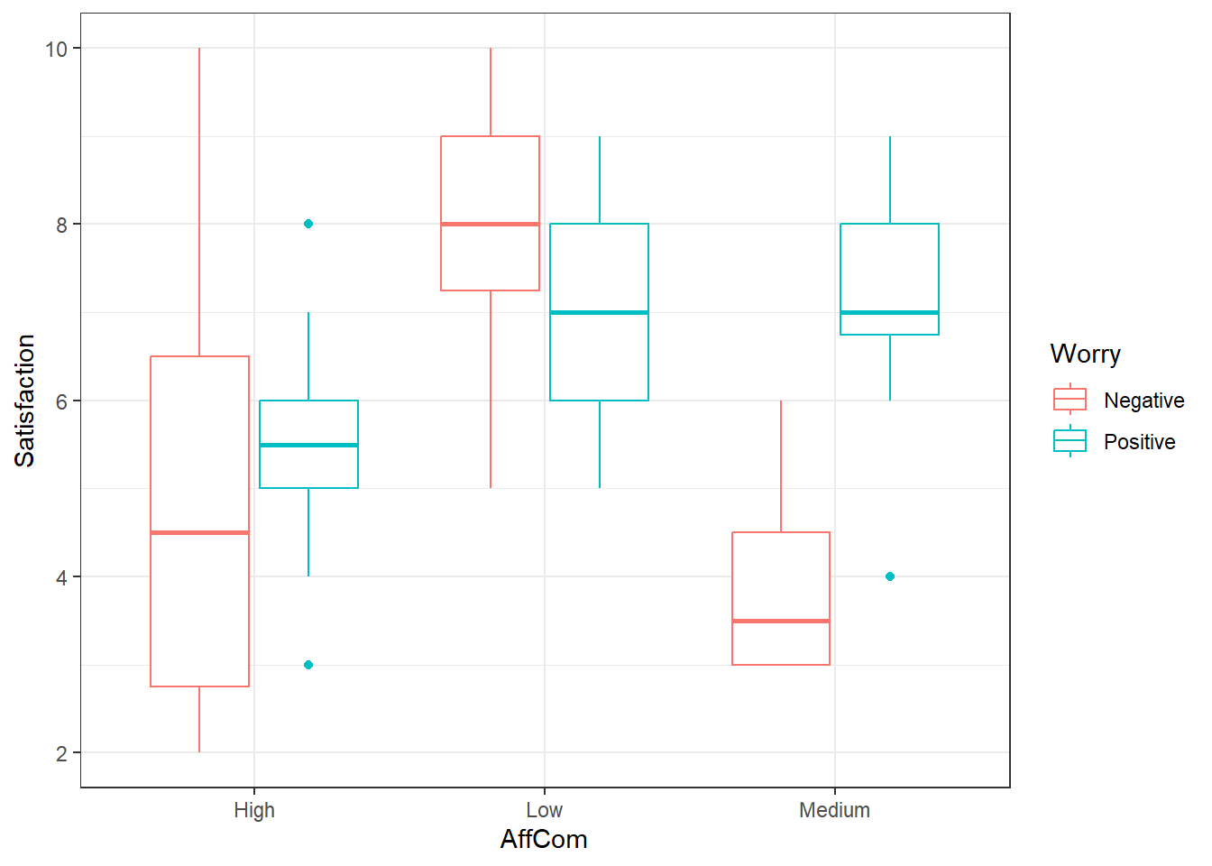

Looks like an interaction. The pattern is different in the negative group versus the positive group.

15.6.3 Type II ANOVA

First, lets use the default of the Anova() function in the car package.

This will do Type II Tests by default

# Make your model
pat.fit <- lm(Satisfaction ~ AffCom*Worry, patSas)

Anova(pat.fit)

Anova Table (Type II tests)

Response: Satisfaction
              Sum Sq Df F value    Pr(>F)    
AffCom        51.829  2  8.3112 0.0008292 ***
Worry          3.425  1  1.0984 0.3000824    
AffCom:Worry  26.682  2  4.2787 0.0197611 *  
Residuals    143.429 46                      
---
Signif. codes:  0 '***' 0.001 '**' 0.01 '*' 0.05 '.' 0.1 ' ' 1

Here we have somewhat strong evidence that there is an interaction.

This wouldn’t fall under my default criteria for declaring “significance” if I were in the NHST frame of reference.
Interaction is fairly apparent from the graphs.
I would err on the side of caution, and declare that there is one.
- We would have to ignore main effects, but if there is actually an interaction, main effect analyses would be difficult to interpret.
- It might be prudent for higher \(\alpha\) values for interaction tests in general.

15.6.4 Type III ANOVA

To do type III ANOVA in R, specifically within the Anova() function, you have to do a couple things.

There is a type argument so you would use Anova(model, type = "III") or type = 3.
You need also need to specify a special option.
Then you have to create a new model AFTER you use that option.
This is usually the default method in most statistical software (other than car in R)

options(contrasts = c("contr.sum","contr.poly"))

pat.fit2 <- lm(Satisfaction ~ AffCom*Worry, patSas)

Anova(pat.fit2, type = 3)

Anova Table (Type III tests)

Response: Satisfaction
              Sum Sq Df  F value    Pr(>F)    
(Intercept)  1679.33  1 538.5911 < 2.2e-16 ***
AffCom         52.11  2   8.3566  0.000802 ***
Worry           8.30  1   2.6627  0.109554    
AffCom:Worry   26.68  2   4.2787  0.019761 *  
Residuals     143.43 46                       
---
Signif. codes:  0 '***' 0.001 '**' 0.01 '*' 0.05 '.' 0.1 ' ' 1

Notice that intercept term there, ignore it. That’s just telling us there is an overall mean that is not zero, which is a pointless piece of information given the scores start at 1.

15.6.5 Multiple Comparisons

Everything is the same as previously when using emmeans() and pairs().

If there is an interaction, then you must use emmeans(model, ~ A:B) or A*B.
When using pairs it is safer to use the adjust = "holm" argument.
- Tukey procedures get more unreliable in the case of unbalanced data.
- This procedure conserves FWER under arbitrary conditions and is better than Bonferroni.

15.6.6 Main Effect Comparisons

If we consider the evidence of interaction to be sufficient to conclude that there is in fact an interaction, it is arguably useless to look at main effects.

Furthermore, we would not look at the Worry main effect means and pairwise comparisons.
This is just for demonstration.

worryMeans <- emmeans(pat.fit, ~ Worry)

worryMeans

 Worry    emmean    SE df lower.CL upper.CL
 Negative   5.67 0.406 46     4.85     6.48
 Positive   6.52 0.334 46     5.85     7.20

Results are averaged over the levels of: AffCom 
Confidence level used: 0.95

pairs(worryMeans)

 contrast            estimate    SE df t.ratio p.value
 Negative - Positive   -0.857 0.525 46  -1.632  0.1096

Results are averaged over the levels of: AffCom

There still was an interaction so this comparison may not be considered worthwhile.

comMeans <- emmeans(pat.fit, ~ AffCom)

comMeans

 AffCom emmean    SE df lower.CL upper.CL
 High     5.29 0.391 46     4.50     6.07
 Low      7.50 0.419 46     6.66     8.34
 Medium   5.50 0.541 46     4.41     6.59

Results are averaged over the levels of: Worry 
Confidence level used: 0.95

pairs(comMeans, adjust = "holm")

 contrast      estimate    SE df t.ratio p.value
 High - Low      -2.214 0.573 46  -3.863  0.0010
 High - Medium   -0.214 0.667 46  -0.321  0.7496
 Low - Medium     2.000 0.684 46   2.924  0.0107

Results are averaged over the levels of: Worry 
P value adjustment: holm method for 3 tests

This indicates that high and medium affective communication were associated with lower patient satisfaction scores.

15.6.7 One Way to Look at Interactions: AffCom by Worry Levels

We may only be interested in how affective communication affects satisfaction when looking at the individual levels of worry.

This is a comparison of cell/interaction means.
However, we are subsetting the comparisons we care about.

comByWorryMeans <- emmeans(pat.fit, ~ AffCom | Worry)

comByWorryMeans

Worry = Negative:
 AffCom emmean    SE df lower.CL upper.CL
 High     5.00 0.624 46     3.74     6.26
 Low      8.00 0.558 46     6.88     9.12
 Medium   4.00 0.883 46     2.22     5.78

Worry = Positive:
 AffCom emmean    SE df lower.CL upper.CL
 High     5.57 0.472 46     4.62     6.52
 Low      7.00 0.624 46     5.74     8.26
 Medium   7.00 0.624 46     5.74     8.26

Confidence level used: 0.95

pairs(comByWorryMeans, adjust = "holm")

Worry = Negative:
 contrast      estimate    SE df t.ratio p.value
 High - Low       -3.00 0.838 46  -3.582  0.0016
 High - Medium     1.00 1.080 46   0.925  0.3599
 Low - Medium      4.00 1.040 46   3.829  0.0012

Worry = Positive:
 contrast      estimate    SE df t.ratio p.value
 High - Low       -1.43 0.783 46  -1.825  0.2233
 High - Medium    -1.43 0.783 46  -1.825  0.2233
 Low - Medium      0.00 0.883 46   0.000  1.0000

P value adjustment: holm method for 3 tests

So it seems that the discrepancy arises when worry levels are categorized as “Negative”
However, even though there is low significance, the same pattern arises in the Worry = Positive group.

15.6.8 Or Maybe: Worry by AffCom Levels

We may only be interested in how affective communication affects satisfaction when looking at the individual levels of worry.

This is a comparison of cell/interaction means.
However, we are subsetting the comparisons we care about.

worryByComMeans <- emmeans(pat.fit, ~ Worry | AffCom)

worryByComMeans

AffCom = High:
 Worry    emmean    SE df lower.CL upper.CL
 Negative   5.00 0.624 46     3.74     6.26
 Positive   5.57 0.472 46     4.62     6.52

AffCom = Low:
 Worry    emmean    SE df lower.CL upper.CL
 Negative   8.00 0.558 46     6.88     9.12
 Positive   7.00 0.624 46     5.74     8.26

AffCom = Medium:
 Worry    emmean    SE df lower.CL upper.CL
 Negative   4.00 0.883 46     2.22     5.78
 Positive   7.00 0.624 46     5.74     8.26

Confidence level used: 0.95

pairs(worryByComMeans, adjust = "holm")

AffCom = High:
 contrast            estimate    SE df t.ratio p.value
 Negative - Positive   -0.571 0.783 46  -0.730  0.4690

AffCom = Low:
 contrast            estimate    SE df t.ratio p.value
 Negative - Positive    1.000 0.838 46   1.194  0.2386

AffCom = Medium:
 contrast            estimate    SE df t.ratio p.value
 Negative - Positive   -3.000 1.080 46  -2.774  0.0080

15.6.9 Another way: All Pairwise Comparison (Throw everything at the wall and see what sticks)

cellMeans <- emmeans(pat.fit, ~ AffCom:Worry)

cellMeans

 AffCom Worry    emmean    SE df lower.CL upper.CL
 High   Negative   5.00 0.624 46     3.74     6.26
 Low    Negative   8.00 0.558 46     6.88     9.12
 Medium Negative   4.00 0.883 46     2.22     5.78
 High   Positive   5.57 0.472 46     4.62     6.52
 Low    Positive   7.00 0.624 46     5.74     8.26
 Medium Positive   7.00 0.624 46     5.74     8.26

Confidence level used: 0.95

pairs(cellMeans, adjust = "holm")

 contrast                          estimate    SE df t.ratio p.value
 High Negative - Low Negative        -3.000 0.838 46  -3.582  0.0115
 High Negative - Medium Negative      1.000 1.080 46   0.925  1.0000
 High Negative - High Positive       -0.571 0.783 46  -0.730  1.0000
 High Negative - Low Positive        -2.000 0.883 46  -2.265  0.2825
 High Negative - Medium Positive     -2.000 0.883 46  -2.265  0.2825
 Low Negative - Medium Negative       4.000 1.040 46   3.829  0.0058
 Low Negative - High Positive         2.429 0.731 46   3.322  0.0229
 Low Negative - Low Positive          1.000 0.838 46   1.194  1.0000
 Low Negative - Medium Positive       1.000 0.838 46   1.194  1.0000
 Medium Negative - High Positive     -1.571 1.000 46  -1.570  0.7400
 Medium Negative - Low Positive      -3.000 1.080 46  -2.774  0.0956
 Medium Negative - Medium Positive   -3.000 1.080 46  -2.774  0.0956
 High Positive - Low Positive        -1.429 0.783 46  -1.825  0.5955
 High Positive - Medium Positive     -1.429 0.783 46  -1.825  0.5955
 Low Positive - Medium Positive       0.000 0.883 46   0.000  1.0000

P value adjustment: holm method for 15 tests

And then you have this mess to summarize. (Cell references are in AffCom:Worry format)

Low:Negative have higher mean scores than High:Negative, High:Positive, and Medium:Negative. (p \(\leq\) 0.0229)
All other comparisons are inconclusive.

A generalization of this is that Low affective communication and Negative worry were associated with higher satisfaction scores.

Hopefully this means that the scale goes from very satisfied to very disatisfied in terms of 1 through 10 and affective communication leads to better satisfaction.
Otherwise if a patient is categorized and “negative” on the worry skill, we should send in a doctor that sucks at communicating, apparently.