# Here are the libraries I used
library(tidyverse) # standard
library(knitr) # need for a couple things to make knitted document to look nice
library(readr) # need to read in data
library(ggpubr) # allows for stat_cor in ggplots
library(ggfortify) # Needed for autoplot to work on lm()
library(gridExtra) # allows me to organize the graphs in a grid
library(car) # need for some regression stuff like vif
library(GGally)
library(Hmisc) # Needed for some visuals
library(rms) # needed for some data reduction tech.
library(pcaPP)
library(see)
library(performance)9 Variable Selection, Data Reduction, and Model Comparison
Here are some code chunks that setup this document.
# This changes the default theme of ggplot
old.theme <- theme_get()
theme_set(theme_bw())
9.1 Explainable statistical learning in public health for policy development: the case of real-world suicide data
We will work with data made available from this paper:
https://bmcmedresmethodol.biomedcentral.com/articles/10.1186/s12874-019-0796-7
If you want to go really in-depth of how you deal with data, this article goes into a lot of detail.
phe <- read_csv(here::here("datasets","phe.csv"))9.1.1 Variables. A LOT!
| Variables |
|---|
| 2014 Suicide (age-standardised rate per 100,000 - outcome measure) |
| 2013 Adult social care users who have as much social contact as they would like (% of adult social care users) |
| 2013 Adults in treatment at specialist alcohol misuse services (rate per 1000 population) |
| 2013 Adults in treatment at specialist drug misuse services (rate per 1000 population) |
| 2013 Alcohol-related hospital admission (female) (directly standardised rate per 100,000 female population) |
| 2013 Alcohol-related hospital admission (male) (directly standardised rate per 100,000 male population) |
| 2013 Alcohol-related hospital admission (directly standardised rate per 100,000 population) |
| 2013 Children in the youth justice system (rate per 1,000 aged 10–18) |
| 2013 Children leaving care (rate per 10,000 < 18 population) |
| 2013 Depression recorded prevalence (% of adults with a new diagnosis of depression who had a bio-psychosocial assessment) |
| 2013 Domestic abuse incidents (rate per 1,000 population) |
| 2013 Emergency hospital admissions for intentional self-harm (female) (directly age-standardised rate per 100,000 women) |
| 2013 Emergency hospital admissions for intentional self-harm (male) (directly age-standardised rate per 100,000 men) |
| 2013 Emergency hospital admissions for intentional self-harm (directly age-and-sex-standardised rate per 100,000) |
| 2013 Looked after children (rate per 10,000 < 18 population) |
| 2013 Self-reported well-being - high anxiety (% of people) |
| 2013 Severe mental illness recorded prevalence (% of practice register [all ages]) |
| 2013 Social care mental health clients receiving services (rate per 100,000 population) |
| 2013 Statutory homelessness (rate per 1000 households) |
| 2013 Successful completion of alcohol treatment (% who do not represent within 6 months) |
| 2013 Successful completion of drug treatment - non-opiate users (% who do not represent within 6 months) |
| 2013 Successful completion of drug treatment - opiate users (% who do not represent within 6 months) |
| 2013 Unemployment (% of working-age population) |
| 2012 Adult carers who have as much social contact as they would like (18+ yrs) (% of 18+ carers) |
| 2012 Adult carers who have as much social contact as they would like (all ages) (% of adult carers) |
| 2011 Estimated prevalence of opiates and/or crack cocaine use (rate per 1,000 aged 15–64) |
| 2011 Long-term health problems or disability (% of people whose day-to-day activities are limited by their health or disability) |
| 2011 Marital breakup (% of adults whose current marital status is separated or divorced) |
| 2011 Older people living alone (% of households occupied by a single person aged 65 or over) |
| 2011 People living alone (% of all households occupied by a single person) |
| Mental Health Service users with crisis plans: % of people in contact with services with a crisis plan in place (end of quarter snapshot) |
| Older people |
| 2011 Self-reported well-being - low happiness (% of people with a low happiness score) |
9.2 How do we choose variables?
Objective: Find a way to predict suicide rates.
We could just use all of the predictors in a linear model.
fullLm <- lm(suicide_rate ~ ., phe)

summary(fullLm)
Call:
lm(formula = suicide_rate ~ ., data = phe)

Residuals:
    Min      1Q  Median      3Q     Max
-3.0118 -1.0447 -0.2702  0.9903  4.1993

Coefficients:
                                 Estimate Std. Error t value Pr(>|t|)
(Intercept)                     2.0155877  3.5059381   0.575    0.566
children_youth_justice         -0.0235629  0.0247292  -0.953    0.343
adult_carers_isolated_18        0.0336685  0.0262501   1.283    0.202
adult_carers_isolated_all_ages -0.0226404  0.0424220  -0.534    0.595
adult_carers_not_isolated       0.3786174  0.2379446   1.591    0.114
alcohol_rx_18                  -0.3001189  0.2515821  -1.193    0.235
alcohol_rx_all_ages            -0.0130574  0.0148093  -0.882    0.380
alcohol_admissions_f           -0.0060296  0.0127911  -0.471    0.638
alchol_admissions_m             0.0167345  0.0268020   0.624    0.534
alcohol_admissions_p           -0.0600782  0.0895445  -0.671    0.504
children_leaving_care           0.0216349  0.0288644   0.750    0.455
depression                     -0.1169805  0.1328876  -0.880    0.380
domestic_abuse                  0.0269278  0.0419236   0.642    0.522
self_harm_female                0.0369915  0.0946913   0.391    0.697
self_harm_male                  0.0318458  0.0944774   0.337    0.737
self_harm_persons              -0.0658812  0.1902674  -0.346    0.730
opiates                         0.2041520  0.1375203   1.485    0.140
lt_health_problems              0.0318830  0.1456081   0.219    0.827
lt_unepmloyment                -0.6342130  1.2588572  -0.504    0.615
looked_after_children           0.0174365  0.0146237   1.192    0.236
marital_breakup                 0.1606036  0.1723378   0.932    0.353
old_pople_alone                 0.3779967  0.4371635   0.865    0.389
alone                          -0.1004305  0.1386281  -0.724    0.470
self_reported_well_being        0.0605038  0.0681410   0.888    0.376
smi                             2.1708482  1.3401643   1.620    0.108
social_care_mh                  0.0006815  0.0005270   1.293    0.199
homeless                       -0.1550536  0.1051424  -1.475    0.143
alcohol_rx                      0.0170587  0.0282631   0.604    0.547
drug_rx_non_opiate             -0.0408008  0.0271119  -1.505    0.135
drug_rx_opiate                  0.1068925  0.0848400   1.260    0.210
unemployment                    0.0690206  0.2925910   0.236    0.814

Residual standard error: 1.687 on 118 degrees of freedom
Multiple R-squared:  0.5031,    Adjusted R-squared:  0.3767
F-statistic: 3.982 on 30 and 118 DF, p-value: 3.823e-08autoplot(fullLm)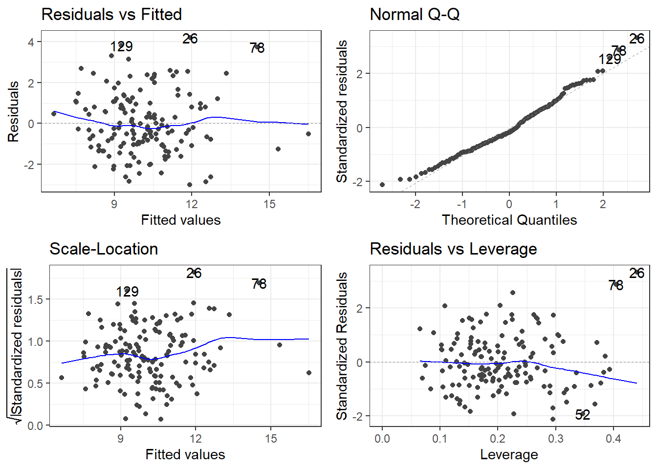
If we are going by statistical significance, each predictor variable fails but the global F-test says that a linear model is working (sort of).
And that \(R^2\) is pretty good for “prediciting” something related to human behavior.
Residuals look good.
Overall, this is bad!
You do not just use all the variables you have
Though there are exceptions: read Harrell’s Regression Model Strategies (Chapter 4, Section 12, 4.12.1 - 4.12.3)
9.2.1 The scope of the problem
How many variables are there to use…? How well do they work?
We could try cor(phe) and see which variables are most correlated with suicide_rate. (You’ll get a lot of output… that’s \(31\times 31 = 961\) correlations)
I’ll save you the pain and just show the correlations with just suicide_rate.
                               suicide_rate
children_youth_justice           0.05847330
adult_carers_isolated_18         0.24939518
adult_carers_isolated_all_ages   0.20369843
adult_carers_not_isolated        0.45228878
alcohol_rx_18                    0.38997284
alcohol_rx_all_ages              0.33117982
alcohol_admissions_f             0.29906808
alchol_admissions_m              0.31868168
alcohol_admissions_p             0.11433511
children_leaving_care            0.36700280
depression                       0.32509700
domestic_abuse                   0.14835220
self_harm_female                 0.49025136
self_harm_male                   0.52004798
self_harm_persons                0.51686092
opiates                          0.41195709
lt_health_problems               0.47825399
lt_unepmloyment                  0.19643927
looked_after_children            0.51243274
marital_breakup                  0.39971208
old_pople_alone                  0.39870200
alone                            0.31037882
self_reported_well_being         0.12949288
smi                              0.18390513
social_care_mh                   0.20125278
homeless                        -0.32105739
alcohol_rx                      -0.07513134
drug_rx_non_opiate              -0.14207504
drug_rx_opiate                  -0.14345307
unemployment                     0.18827138
9.2.2 Just use the best correlations?
These are a few of the strongest correlations.
                               suicide_rate

self_harm_female                 0.49025136
self_harm_male                   0.52004798
self_harm_persons                0.51686092
looked_after_children            0.51243274
Let’s make a model.
badIdea <- lm(suicide_rate ~ self_harm_female + self_harm_male + self_harm_persons + looked_after_children, phe)

summary(badIdea)
Call:
lm(formula = suicide_rate ~ self_harm_female + self_harm_male +
    self_harm_persons + looked_after_children, data = phe)

Residuals:
    Min      1Q  Median      3Q     Max
-4.1974 -1.2196  0.0677  1.1319  6.4354

Coefficients:
                       Estimate Std. Error t value Pr(>|t|)
(Intercept)            6.521275   0.485989  13.419  < 2e-16 ***
self_harm_female       0.059297   0.087465   0.678 0.498889
self_harm_male         0.053601   0.087682   0.611 0.541954
self_harm_persons     -0.106747   0.175961  -0.607 0.545038
looked_after_children  0.031342   0.008442   3.713 0.000292 ***
---
Signif. codes:  0 '***' 0.001 '**' 0.01 '*' 0.05 '.' 0.1 ' ' 1

Residual standard error: 1.763 on 144 degrees of freedom
Multiple R-squared:  0.3379,    Adjusted R-squared:  0.3195
F-statistic: 18.37 on 4 and 144 DF,  p-value: 3.246e-12
What does the model have to say about how the self harm variables are related to suicide rate?
9.3 Multicollinearity
pairs(suicide_rate ~ self_harm_persons + self_harm_female + self_harm_male, phe)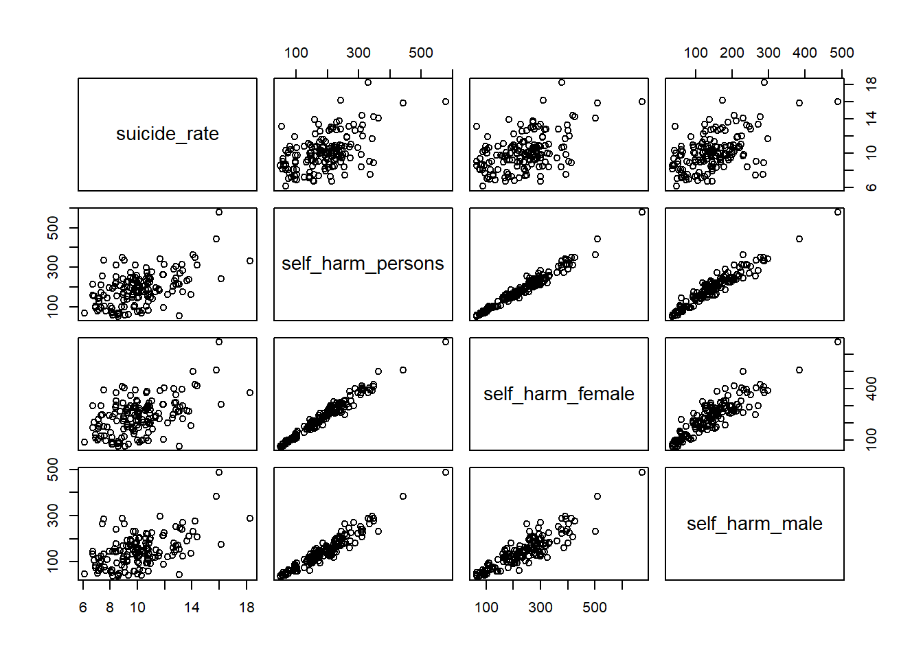
cor(phe$self_harm_female,phe$self_harm_male)[1] 0.8865727cor(phe$self_harm_persons,phe$self_harm_male)[1] 0.9601094cor(phe$self_harm_persons,phe$self_harm_female)[1] 0.9804772When we have predictor variables that are linearly related to each other, we have what is called multi-collinearity.
These variables essentially all contribute the same information over and over to the model. This makes a feedback loop that kicks everything around.
What about a model with just self_harm_persons (Why that one?) and looked_after_children?
notAsBadLm <- lm(suicide_rate ~ self_harm_persons + looked_after_children, phe)

summary(notAsBadLm)
Call:
lm(formula = suicide_rate ~ self_harm_persons + looked_after_children,
    data = phe)

Residuals:
    Min      1Q  Median      3Q     Max
-4.3450 -1.2323  0.0677  1.0792  6.2763

Coefficients:
                      Estimate Std. Error t value Pr(>|t|)
(Intercept)           6.704515   0.430054  15.590  < 2e-16 ***
self_harm_persons     0.008385   0.002124   3.947 0.000123 ***
looked_after_children 0.027803   0.007281   3.818 0.000198 ***
---
Signif. codes:  0 '***' 0.001 '**' 0.01 '*' 0.05 '.' 0.1 ' ' 1

Residual standard error: 1.756 on 146 degrees of freedom
Multiple R-squared:  0.3337,    Adjusted R-squared:  0.3246
F-statistic: 36.56 on 2 and 146 DF,  p-value: 1.344e-13
9.3.1 But what about self harm and looking after children?
Relations may not be as blaringly obvious as that. What about self harm and looking after children?
ggplot(phe, aes(x = self_harm_persons, y = looked_after_children)) +
  geom_point() +
  stat_cor()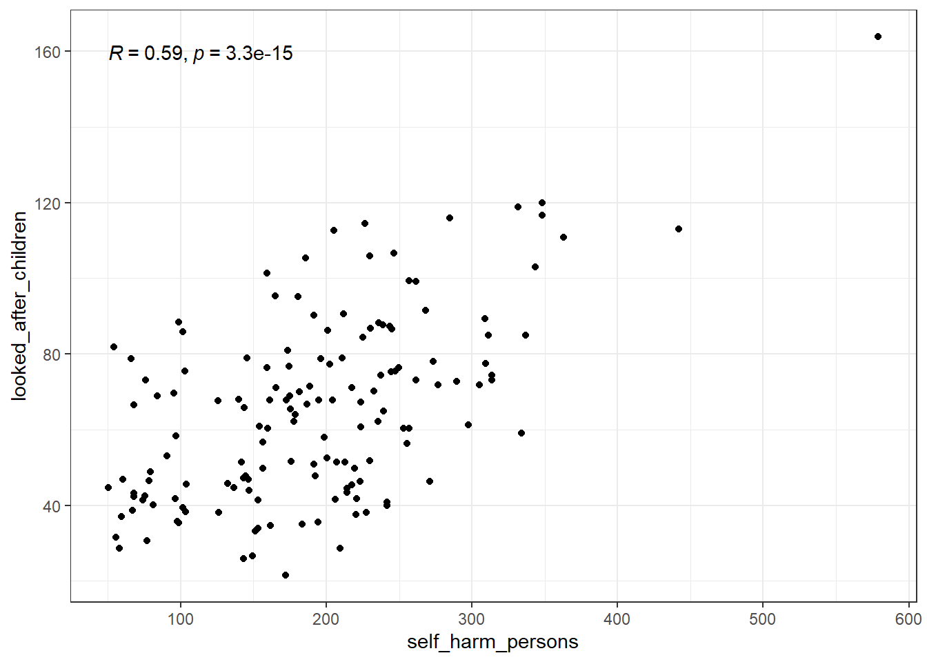
This isn’t nearly as bad and wouldn’t be considered a detrimental relation.
9.4 Measuring multi-collinearity
9.4.1 A linear model for the predictors
Linear relation between many predictor variables.
\[x_k =\beta_{0}^* + \beta_{1}^* x_1 + \beta_{2}^*x_2 + \dots + \beta_p^* x_p + \epsilon^*\]
This is like any model and has it’s own \(R^2\) \(R^2_k\).
If this \(R^2\) is high, it means that a predictor variable is redundant.
There are a few ways to measure “high”.
Some sources would say that \(0.8 \le R_k^2 \le 0.9\) would be problematic, and you have extreme multicollinearity issues for anything higher.
9.4.2 Tolerance
Tolerance is \(1 - R^2_k\).
That’s it.
So \(0.2\) is the “problematic” cutoff and \(0.9\) is the “extreme” cutoff.
It may be referred to as TOL sometimes.
9.4.3 Variance Inflation Factors
The Variance Inflation Factor is:
\[VIF_k = \frac{1}{1 - R^2_k}\]
The VIF is considered “problematic” if greater than 5, and “extreme” if greater than 10.
9.4.4 Getting TOL or VIF: performance package
A nifty package that will help us deal with all the nasty bits of linear regression in R is the performance package. It is part of the easystats universe of packages.
To get tolerance and VIFs, create the model using lm(), and then plug it into the check_collinearity function.
check_collinearity(model)
library(performance)
library(see)

# badidea was the model with all the self harm variables

check_collinearity(badIdea)
# Check for Multicollinearity
Low Correlation
Term VIF VIF 95% CI Increased SE Tolerance
looked_after_children 2.04 [ 1.66, 2.63] 1.43 0.49
Tolerance 95% CI
[0.38, 0.60]
High Correlation
Term VIF VIF 95% CI Increased SE Tolerance
self_harm_female 3811.50 [2809.27, 5171.42] 61.74 2.62e-04
self_harm_male 1863.65 [1373.68, 2528.51] 43.17 5.37e-04
self_harm_persons 10400.43 [7665.39, 14111.48] 101.98 9.61e-05
Tolerance 95% CI
[0.00, 0.00]
[0.00, 0.00]
[0.00, 0.00]Versus
check_collinearity(notAsBadLm)# Check for Multicollinearity
Low Correlation
Term VIF VIF 95% CI Increased SE Tolerance
self_harm_persons 1.53 [1.29, 1.96] 1.24 0.65
looked_after_children 1.53 [1.29, 1.96] 1.24 0.65
Tolerance 95% CI
[0.51, 0.78]
[0.51, 0.78]9.4.5 Plot check_collinearity checks
plot(check_collinearity(badIdea))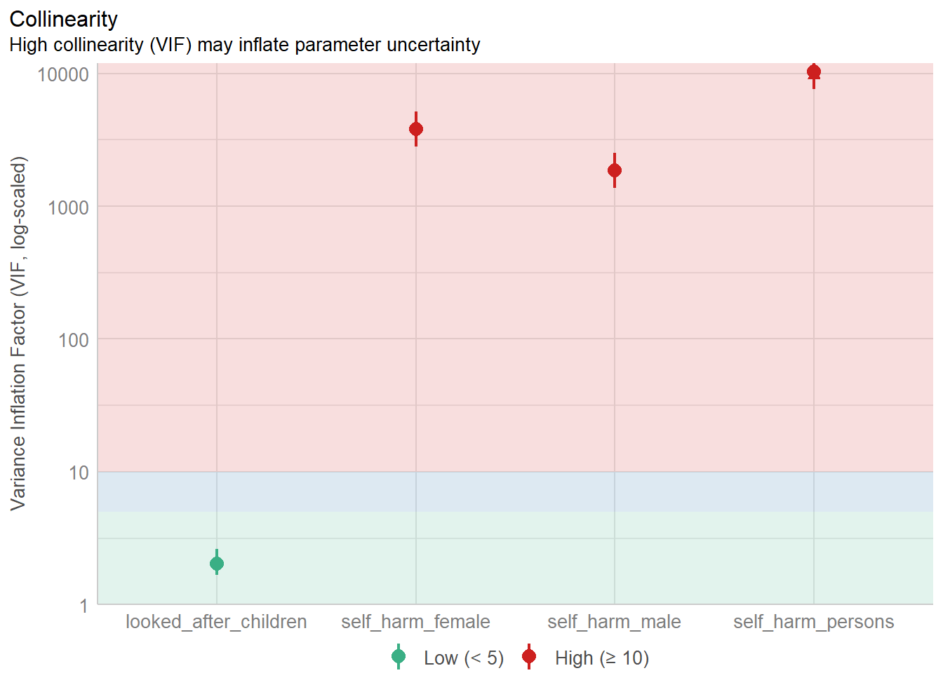
Versus
plot(check_collinearity(notAsBadLm))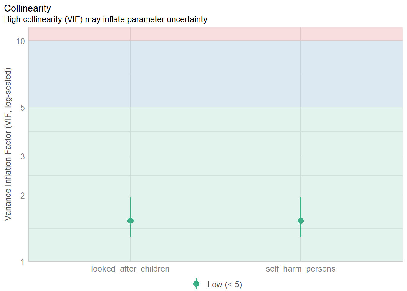
9.4.6 VIF and Tolerance in the full model
You do not get rid of a variable because it has a small tolerance/large VIF!
You would investigate which variables are most correlated with eachother.
You need to use your own reasoning to decide which variables to remove based on the correlations between predictors AND the response.
Tolerance and VIF only indicate that the overall model has a problem, not the individual variable.
check_collinearity(fullLm)# Check for Multicollinearity
Low Correlation
Term VIF VIF 95% CI Increased SE
children_youth_justice 1.48 [ 1.29, 1.80] 1.22
adult_carers_isolated_18 1.88 [ 1.59, 2.30] 1.37
adult_carers_isolated_all_ages 1.84 [ 1.57, 2.26] 1.36
adult_carers_not_isolated 3.11 [ 2.55, 3.88] 1.76
alcohol_admissions_p 2.05 [ 1.73, 2.52] 1.43
children_leaving_care 4.32 [ 3.49, 5.42] 2.08
depression 2.73 [ 2.25, 3.38] 1.65
domestic_abuse 1.90 [ 1.61, 2.33] 1.38
marital_breakup 2.36 [ 1.97, 2.91] 1.54
alone 4.82 [ 3.88, 6.06] 2.19
self_reported_well_being 1.42 [ 1.24, 1.72] 1.19
smi 3.62 [ 2.94, 4.52] 1.90
social_care_mh 1.29 [ 1.15, 1.58] 1.14
homeless 3.11 [ 2.55, 3.87] 1.76
alcohol_rx 3.27 [ 2.68, 4.08] 1.81
drug_rx_non_opiate 3.21 [ 2.63, 4.00] 1.79
drug_rx_opiate 1.99 [ 1.68, 2.44] 1.41
Tolerance Tolerance 95% CI
0.68 [0.56, 0.78]
0.53 [0.43, 0.63]
0.54 [0.44, 0.64]
0.32 [0.26, 0.39]
0.49 [0.40, 0.58]
0.23 [0.18, 0.29]
0.37 [0.30, 0.44]
0.53 [0.43, 0.62]
0.42 [0.34, 0.51]
0.21 [0.16, 0.26]
0.71 [0.58, 0.81]
0.28 [0.22, 0.34]
0.77 [0.63, 0.87]
0.32 [0.26, 0.39]
0.31 [0.24, 0.37]
0.31 [0.25, 0.38]
0.50 [0.41, 0.60]
Moderate Correlation
Term VIF VIF 95% CI Increased SE Tolerance
lt_unepmloyment 5.30 [ 4.26, 6.68] 2.30 0.19
looked_after_children 6.68 [ 5.33, 8.45] 2.58 0.15
unemployment 8.68 [ 6.89, 11.02] 2.95 0.12
Tolerance 95% CI
[0.15, 0.23]
[0.12, 0.19]
[0.09, 0.15]
High Correlation
Term VIF VIF 95% CI Increased SE Tolerance
alcohol_rx_18 18.48 [ 14.52, 23.59] 4.30 0.05
alcohol_rx_all_ages 351.34 [ 273.84, 450.86] 18.74 2.85e-03
alcohol_admissions_f 978.20 [ 762.20, 1255.50] 31.28 1.02e-03
alchol_admissions_m 2345.59 [ 1827.47, 3010.68] 48.43 4.26e-04
self_harm_female 4877.78 [ 3800.20, 6261.00] 69.84 2.05e-04
self_harm_male 2362.51 [ 1840.66, 3032.40] 48.61 4.23e-04
self_harm_persons 13277.66 [10344.20, 17043.10] 115.23 7.53e-05
opiates 12.46 [ 9.83, 15.87] 3.53 0.08
lt_health_problems 11.71 [ 9.25, 14.91] 3.42 0.09
old_pople_alone 11.18 [ 8.84, 14.23] 3.34 0.09
Tolerance 95% CI
[0.04, 0.07]
[0.00, 0.00]
[0.00, 0.00]
[0.00, 0.00]
[0.00, 0.00]
[0.00, 0.00]
[0.00, 0.00]
[0.06, 0.10]
[0.07, 0.11]
[0.07, 0.11]You have to jump through a lot of hoops and then make justifiable choices.
9.4.7 Detecting Multicollinearity
The following our indicators of multicollinearity:
- “Significant” correlations between pairs of independent variables.
- Non-significant t-tests for all or nearly all of the predictor variables, but a significant global F-test.
- The coefficients have opposite signs than what would be expected (by logic or compared to the individual correlation with the response variable).
- A single VIF of 10, more than one VIF of 5 or above. Several VIF 3 or over. Or corresponding tolerance values. Or corresponding \(R^2_k\) values
The cutoffs for VIF, tolerance, or \(R^2_k\) are guidelines not solid rules. Theory should always trump these more arbitrary statistical rules.
9.5 Variable screening the PHE data
The paper has various methods for variable selection to remove multicollinearity issues.
They don’t really document it that well… Here’s my best take.
# I created this dataset after going through things over and over
# I removed variables from the csv as I was working with it in R
# Lots of fun!

# also, I only use this dataset for demonstration so I don't have to type out
# all of the variables I left in the data into the formula.

pheRed <- read_csv(here::here("datasets",
                              'phe_reduced.csv'))

redModel <- lm(suicide_rate ~ ., pheRed)

check_collinearity(redModel)
# Check for Multicollinearity
Low Correlation
Term VIF VIF 95% CI Increased SE Tolerance
children_youth_justice 1.13 [1.04, 1.51] 1.06 0.88
adult_carers_isolated_all_ages 1.48 [1.27, 1.85] 1.22 0.68
alcohol_admissions_p 1.78 [1.49, 2.23] 1.33 0.56
children_leaving_care 2.58 [2.09, 3.30] 1.61 0.39
depression 2.21 [1.81, 2.80] 1.49 0.45
domestic_abuse 1.42 [1.23, 1.78] 1.19 0.70
self_harm_persons 2.35 [1.92, 2.99] 1.53 0.43
opiates 2.14 [1.76, 2.70] 1.46 0.47
marital_breakup 1.83 [1.53, 2.30] 1.35 0.55
alone 1.49 [1.28, 1.87] 1.22 0.67
self_reported_well_being 1.24 [1.10, 1.57] 1.11 0.81
social_care_mh 1.17 [1.05, 1.51] 1.08 0.86
homeless 2.25 [1.84, 2.86] 1.50 0.44
alcohol_rx 1.43 [1.24, 1.80] 1.20 0.70
drug_rx_opiate 1.62 [1.37, 2.03] 1.27 0.62
Tolerance 95% CI
[0.66, 0.97]
[0.54, 0.79]
[0.45, 0.67]
[0.30, 0.48]
[0.36, 0.55]
[0.56, 0.81]
[0.33, 0.52]
[0.37, 0.57]
[0.43, 0.65]
[0.54, 0.78]
[0.64, 0.91]
[0.66, 0.95]
[0.35, 0.54]
[0.56, 0.81]
[0.49, 0.73]Some variables I removed because I could not find the correct definition.
I am not an expert on this stuff so I had to do my best based on my mediocre knowledge of the subject matter, and trying to figure out what the authors of the paper were saying.
When it is okay to stop removing variables is entirely dependent on the situation. I don’t even have a guideline for it.
9.6 Next step: Choosing an actual model
Supposing the multicollinearity issue has been solved, how do we move on?
Do we use all the variables in the model?
summary(redModel)
Call:
lm(formula = suicide_rate ~ ., data = pheRed)

Residuals:
    Min      1Q  Median      3Q     Max
-3.8689 -1.1154 -0.0917  0.8901  4.2030

Coefficients:
                                 Estimate Std. Error t value Pr(>|t|)
(Intercept)                     4.0832859  3.0285950   1.348   0.1799
children_youth_justice         -0.0136101  0.0220822  -0.616   0.5387
adult_carers_isolated_all_ages  0.0000509  0.0387482   0.001   0.9990
alcohol_admissions_p           -0.0623441  0.0849678  -0.734   0.4644
children_leaving_care           0.0422261  0.0227752   1.854   0.0659 .
depression                     -0.1622739  0.1220073  -1.330   0.1858
domestic_abuse                  0.0247253  0.0369822   0.669   0.5049
self_harm_persons               0.0066734  0.0025813   2.585   0.0108 *
opiates                         0.1010386  0.0580642   1.740   0.0842 .
marital_breakup                 0.2937180  0.1548091   1.897   0.0600 .
alone                           0.0336382  0.0786620   0.428   0.6696
self_reported_well_being        0.0345748  0.0650050   0.532   0.5957
social_care_mh                  0.0007603  0.0005101   1.490   0.1385
homeless                       -0.2377671  0.0912485  -2.606   0.0102 *
alcohol_rx                     -0.0047326  0.0190770  -0.248   0.8045
drug_rx_opiate                  0.0305590  0.0779842   0.392   0.6958
---
Signif. codes:  0 '***' 0.001 '**' 0.01 '*' 0.05 '.' 0.1 ' ' 1

Residual standard error: 1.72 on 133 degrees of freedom
Multiple R-squared:  0.4176,    Adjusted R-squared:  0.3519
F-statistic: 6.358 on 15 and 133 DF,  p-value: 5.163e-10
Well now at least some of the predictor’s are significant.
We should not just use all predictors since that ruins the generalizibility of the model.
9.6.0.1 The principle of parsimony: Models should have as few variables/parameters as possible while retaining adequacy.
9.7 Methods for model assessment
We have many variables to choose from, and it’s really easy to make a model.
Should we just pick the variables most highly correlated with suicide rate?
What is our cutoff then?
                               suicide_rate
children_youth_justice           0.05847330
adult_carers_isolated_all_ages   0.20369843
alcohol_admissions_p             0.11433511
children_leaving_care            0.36700280
depression                       0.32509700
domestic_abuse                   0.14835220
self_harm_persons                0.51686092
opiates                          0.41195709
marital_breakup                  0.39971208
alone                            0.31037882
self_reported_well_being         0.12949288
social_care_mh                   0.20125278
homeless                        -0.32105739
alcohol_rx                      -0.07513134
drug_rx_opiate                  -0.14345307
cor1 <- lm(suicide_rate ~ self_harm_persons, phe)
cor2 <- lm(suicide_rate ~ self_harm_persons + opiates, phe)
cor3 <- lm(suicide_rate ~ self_harm_persons + opiates + marital_breakup, phe)
cor4 <- lm(suicide_rate ~ self_harm_persons + opiates + marital_breakup +
children_leaving_care, phe)
cor5 <- lm(suicide_rate ~ self_harm_persons + opiates + marital_breakup +
children_leaving_care + depression, phe)
cor6 <- lm(suicide_rate ~ self_harm_persons + opiates + marital_breakup +
children_leaving_care + depression + homeless, phe)- Is the last model the best?
- Should we add more variables?
- Different variables?
9.7.1 Just “significant” variables?
Lets use any of the variables that had a p-value below 0.1.
# Changing model name method since now we will be looking at several models

sig1 <- lm(suicide_rate ~ children_leaving_care + self_harm_persons + opiates + marital_breakup + homeless, phe)

summary(sig1)
Call:
lm(formula = suicide_rate ~ children_leaving_care + self_harm_persons +
    opiates + marital_breakup + homeless, data = phe)

Residuals:
    Min      1Q  Median      3Q     Max
-3.8194 -1.1301 -0.1541  0.9383  5.6420

Coefficients:
                       Estimate Std. Error t value Pr(>|t|)
(Intercept)            4.855937   1.449776   3.349  0.00104 **
children_leaving_care  0.037193   0.019703   1.888  0.06109 .
self_harm_persons      0.005501   0.002307   2.385  0.01840 *
opiates                0.123432   0.050315   2.453  0.01536 *
marital_breakup        0.218171   0.134664   1.620  0.10741
homeless              -0.212926   0.075547  -2.818  0.00551 **
---
Signif. codes:  0 '***' 0.001 '**' 0.01 '*' 0.05 '.' 0.1 ' ' 1

Residual standard error: 1.705 on 143 degrees of freedom
Multiple R-squared:  0.385, Adjusted R-squared:  0.3635
F-statistic: 17.91 on 5 and 143 DF, p-value: 9.201e-14autoplot(sig1)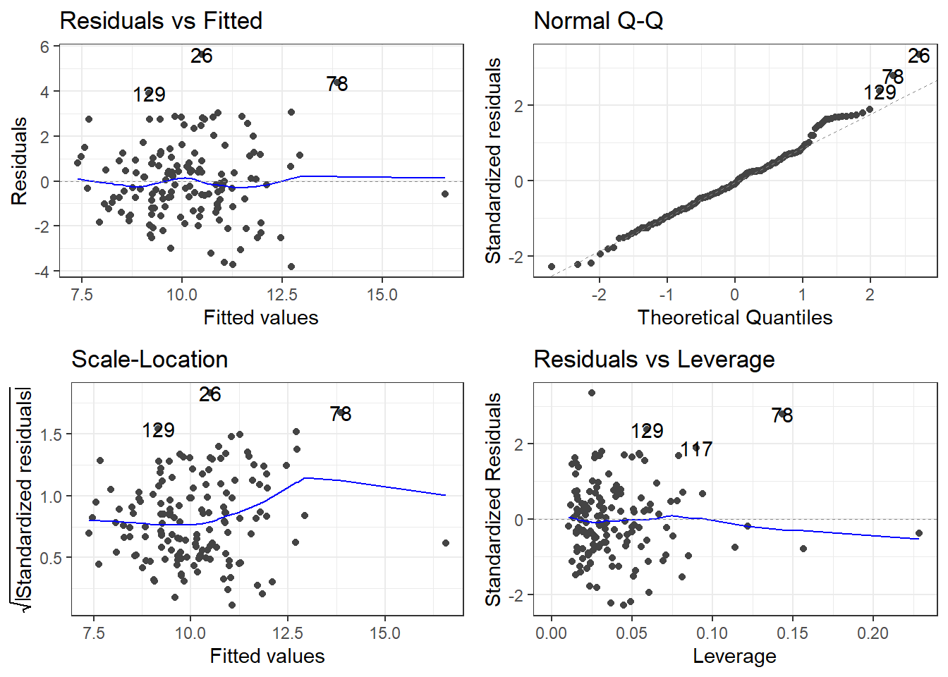
Wait… now marital breakup isn’t significant?
# Changing model name method since now we will be looking at several models

sig2 <- lm(suicide_rate ~ children_leaving_care + self_harm_persons + opiates +
             homeless, phe)

summary(sig2)
Call:
lm(formula = suicide_rate ~ children_leaving_care + self_harm_persons +
    opiates + homeless, data = phe)

Residuals:
    Min      1Q  Median      3Q     Max
-3.8777 -1.1053  0.0011  1.0022  5.8723

Coefficients:
                       Estimate Std. Error t value Pr(>|t|)
(Intercept)            7.033367   0.546679  12.866  < 2e-16 ***
children_leaving_care  0.044142   0.019338   2.283  0.02392 *
self_harm_persons      0.006671   0.002203   3.028  0.00292 **
opiates                0.121234   0.050580   2.397  0.01782 *
homeless              -0.227131   0.075459  -3.010  0.00309 **
---
Signif. codes:  0 '***' 0.001 '**' 0.01 '*' 0.05 '.' 0.1 ' ' 1

Residual standard error: 1.714 on 144 degrees of freedom
Multiple R-squared:  0.3738,    Adjusted R-squared:  0.3564
F-statistic: 21.49 on 4 and 144 DF, p-value: 6.473e-14autoplot(sig2)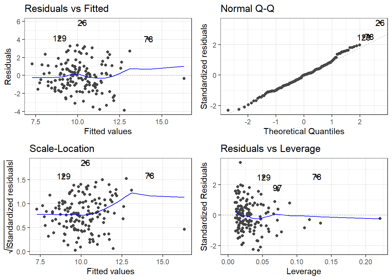
- Relying on “statistical” significance means you will end-up shooting yourself in the foot, metaphorically speaking, i.e., make a bad model.
9.7.2 \(R^2\)? (Don’t use it to choose models).
Recall the definition of \(R^2\): It is the proportion of variability in the response variable explained by your predictor variables in the linear model.
Higher \(R^2\) is better, so maybe we should choose the model with the highest \(R^2\)?
- The full model has an \(R^2\) of 0.5031.
- After whittling down some variables due to multicollinearity,
model1has an \(R^2\) of 0.385. model2has an \(R^2\) of 0.3738.
So the full model is best! Right? All this stuff about variable elimination is pointless. I wasted hours of my life to get to this point…. No!
Never determine which is the best model via \(R^2\).
- \(R^2\) can be arbitrarily high when using many variables that may not be actually related to the response variable in any meaningful way.
n = 500
a = 10; b = 10

### MAKING DATA WITH A TRUE LINEAR MODEL
x <- rnorm(n, 10, 5)
y = a + b*x + rnorm(n,0 ,80)

data <- data.frame(y,x)

ggplot(data, aes(x,y)) +
  geom_point() +
  geom_smooth(method = 'lm')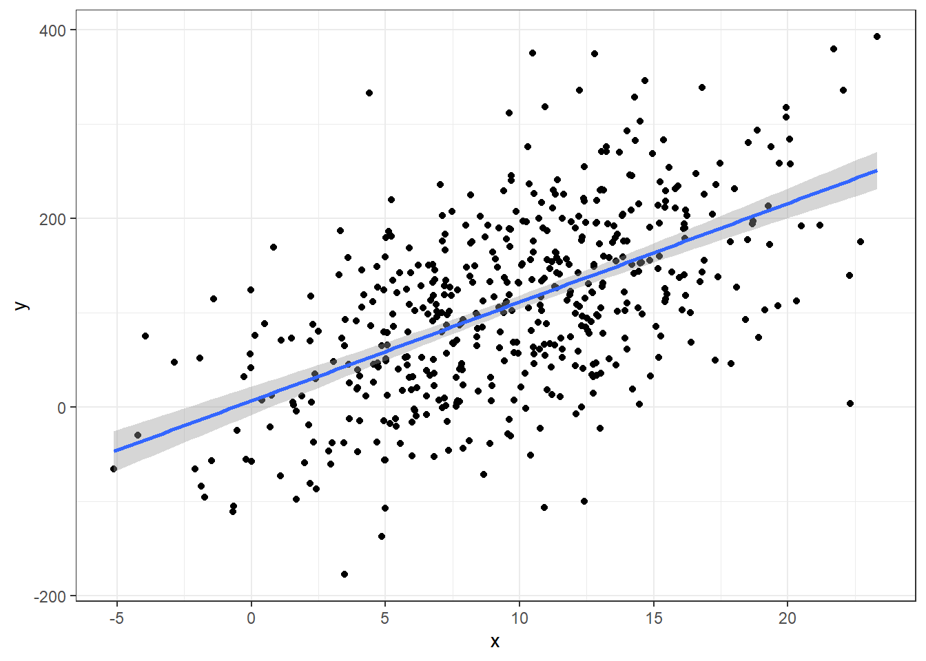
summary(lm(y ~ x, data))
Call:
lm(formula = y ~ x, data = data)

Residuals:
     Min       1Q   Median       3Q      Max
-236.281  -55.592   -0.191   55.531  279.861

Coefficients:
            Estimate Std. Error t value Pr(>|t|)
(Intercept)   6.7071     7.6542   0.876    0.381
x            10.4567     0.6974  14.994   <2e-16 ***
---
Signif. codes:  0 '***' 0.001 '**' 0.01 '*' 0.05 '.' 0.1 ' ' 1

Residual standard error: 79.85 on 498 degrees of freedom
Multiple R-squared:  0.311, Adjusted R-squared:  0.3096
F-statistic: 224.8 on 1 and 498 DF,  p-value: < 2.2e-16
The R-squared here for the perfectly correct model is 0.3110227
- R-squared can be low even when you use the “correct” model.
Now let’s throw in some irrelevant data and graph what happens to R-squared.
# Extra worthless predictors

p = 300

extra.predictors <- data.frame(matrix(rnorm(n*p), nrow=n))

full.data <- data.frame(data, extra.predictors)# need code to combine true and extra data

rsq = rep(NA, p+1)

for(iter in 1:(p+1)){
form <-formula(paste('y ~ ', paste(names(full.data)[2:(iter+1)], collapse=' + ')))
fit.mdl <- lm(form, data=full.data)
rsq[iter] <- summary(fit.mdl)$r.squared # Get the rsq value for the model.
}
ggplot(data.frame(nvars=1:(p+1), rsq),aes(x=nvars,y=rsq)) +
geom_path()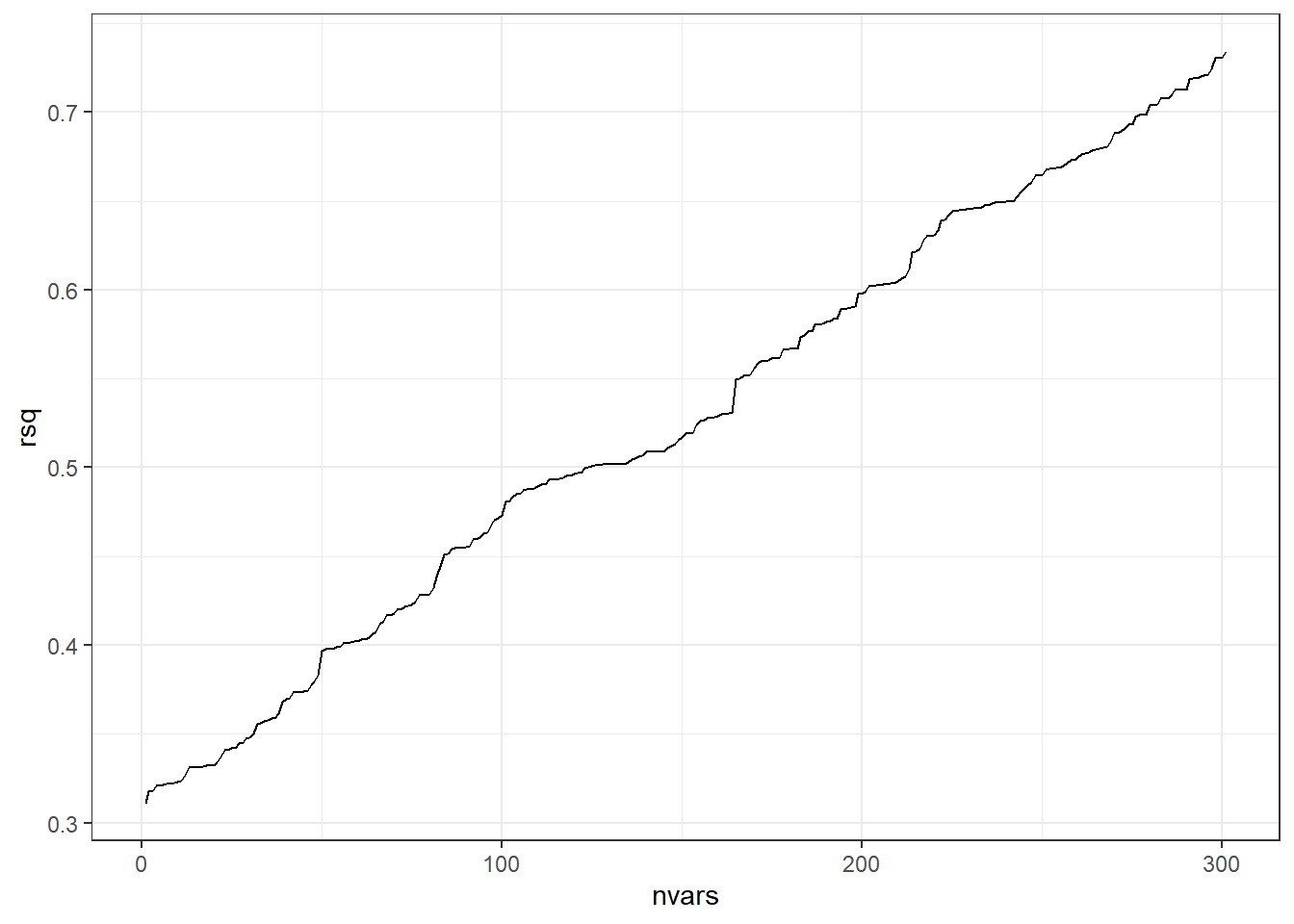
The beginning of the line on the left represents the R-squared value when using the one predictor variable that actually has any true relation with the response variable.
When we add on additional predictors (useless ones), R-squared always increases.
9.7.3 Adjusted \(R^2\) (More conservative)
\[R^2_{adj} = 1 - (1-R^2)\frac{n-1}{n-p-1}\] This is supposed to correct for the fact that \(R^2\) always increases with a greater number of variables (penalizes for the complexity of the model).
Here’s a table for most of the models we’ve discussed so far. It has both the adjusted and unadjusted form.
     model       Rsq    AdjRsq
1   fullLm 0.5030783 0.3767423
2 redModel 0.4176079 0.3519246
3     cor1 0.2671452 0.2621598
4     cor2 0.3275478 0.3183361
5     cor3 0.3476621 0.3341654
6     cor4 0.3508866 0.3328556
7     cor5 0.3514271 0.3287497
8     cor6 0.3943409 0.3687496
But… it doesn’t necessarily. Don’t trust it either.
9.7.4 Predicted \(R^2\) (Even more conservative)
Predicted R-squared or as I will write \(R^2{pred}\) is another play on the same idea as \(R^2\), except for it is based on taking out an observation, computing the regression model without it, then seeing how well the model predicts the left out value.
You can get it via the olsrr package using the ols_pred_rsq() function. The input is your model.
For instance, let us compare this to \(R^2\) from the performance package.
r2(fullLm)# R2 for Linear Regression
R2: 0.503
adj. R2: 0.377library(olsrr)
ols_pred_rsq(fullLm)[1] 0.1258262That’s a lot worse than the 0.503 for the unadjusted R-Squared
Here’s a new table including predicted R-squared
     model       Rsq    AdjRsq   PredRsq
1   fullLm 0.5030783 0.3767423 0.1258262
2 redModel 0.4176079 0.3519246 0.2264297
3     cor1 0.2671452 0.2621598 0.2445699
4     cor2 0.3275478 0.3183361 0.2929179
5     cor3 0.3476621 0.3341654 0.3003604
6     cor4 0.3508866 0.3328556 0.2948558
7     cor5 0.3514271 0.3287497 0.2818233
8 cor6 0.3943409 0.3687496 0.3218613- \(R^2\) only tells how well the model works on the data you have (overfitting kills its utility).
- \(R^2_{adj}\) tries to make an attempt at saying how well the model would work on the wider population/future observations.
- \(R^2_{pred}\) is probably the best measure of how well your model will actually work with new data.
- NONE of these are perfect so use these tools with caution and care.
9.7.5 Akaike Information Criterion AIC
One last point of discussion will be the Akaike Information Criterion.
\[AIC = 2(p+1) + n\log(SSE/n) - C\]
There’s a lot of theory behind this one and the Bayesian Information Criterion (BIC)
\[BIC = (p+1)\ln(n) + n\log(SSE/n) - C\]
This is where things get more confusing since AIC and BIC are numbers where SMALLER IS BETTER.
We will just be looking at AIC
     model       Rsq    AdjRsq   PredRsq      AIC
1   fullLm 0.5030783 0.3767423 0.1258262 183.0882
2 redModel 0.4176079 0.3519246 0.2264297 176.7362
3     cor1 0.2671452 0.2621598 0.2445699 182.9770
4     cor2 0.3275478 0.3183361 0.2929179 172.1605
5     cor3 0.3476621 0.3341654 0.3003604 169.6356
6     cor4 0.3508866 0.3328556 0.2948558 170.8973
7     cor5 0.3514271 0.3287497 0.2818233 172.7732
8     cor6 0.3943409 0.3687496 0.3218613 164.5730
Different measures will tell you different things.
Here \(R^2_{pred}\) and AIC agree that the cor6 model is the best.
cor6 <- lm(suicide_rate ~ self_harm_persons + opiates + marital_breakup +
             children_leaving_care + depression + homeless, phe)
So is that the one we use?
It’s not that simple.
9.8 Variable Selection Methods: Problems and Pitfalls
- Variable selection = methods for choosing which predictor variables to include in statistical models
- Focus on stepwise regression as a common but problematic approach
- Stepwise selection: automated process of adding/removing variables based on statistical significance (p-values and model fit)
9.8.1 Major Problems with Stepwise Selection
9.8.1.1 1. Biased R-squared Values
- R-squared values are inflated
- Makes model appear to explain more variation than it actually does
- Gives false confidence in model’s predictive ability
9.8.1.2 2. Invalid Statistical Inference
- P-values are too small (not valid)
- Confidence intervals are too narrow
- Doesn’t account for multiple testing problem
- Standard errors are biased low
9.8.1.3 3. Biased Regression Coefficients
- Coefficients are biased away from zero
- More likely to select variables with overestimated effects
- Selection process favors chance findings
- True effects may be much smaller than estimated
9.8.1.4 4. Model Instability
- Results highly dependent on sample
- Small changes in data can lead to different variables being selected
- Poor reproducibility
- Different samples likely to produce different models
9.8.2 Example: House Price Prediction
- Scenario: 20 potential predictors of house prices
- First sample might select:
- Square footage
- Number of bathrooms
- Lot size
- Second sample might select completely different variables:
- Age of house
- Number of bedrooms
- Distance to downtown
- Demonstrates instability of selection process
9.8.3 Better Alternatives
9.8.3.1 1. Theory-Driven Selection
- Use subject matter knowledge
- Select variables based on theoretical importance
- Include known important predictors regardless of significance
9.8.3.2 2. Include More Variables
- Keep theoretically important variables
- Don’t eliminate based solely on statistical significance
- Better to include too many than too few important variables
- Degrees of freedom permitting of course!
9.8.3.3 3. Alternative Dimension Reduction Methods
- Principal Components Analysis
- Regularization methods (LASSO, Ridge regression)
- Data reduction techniques that don’t use outcome variable
9.8.4 Key Takeaways
- Avoid automated variable selection methods
- Don’t let computational convenience override good statistical practice
- Complex but theoretically sound models preferred over overly simplified ones
- Statistical significance shouldn’t be the sole criterion for variable inclusion
10 Prespecification of Predictor Complexity in Statistical Modeling
10.1 I. Introduction to Linear Relationships
- Truly linear relationships are rare in real-world data
- Notable exception: Same measurements at different timepoints
- Example: Blood pressure before and after treatment
- Most relationships between predictors and outcomes are nonlinear
- Linear modeling often chosen due to data limitations, not reality
10.2 Problems with Post-Hoc Simplification
10.2.1 Common but Problematic Approaches:
- Examining scatter plots
- Checking descriptive statistics
- Using informal assessments
- Modifying model based on these observations
10.2.2 Key Issue:
- Creates “phantom degrees of freedom”
- Informal assessments use degrees of freedom not accounted for in:
- Standard errors
- P-values
- R² values
10.3 The Prespecification Approach
10.3.1 Core Principles:
- Decide on predictor complexity before examining relationships
- Base decisions on:
- Effective sample size
- Prior knowledge
- Expected predictor importance
- Maintain decisions regardless of analysis results
10.3.2 Benefits:
- More reliable statistical inference
- Better representation of uncertainty
- Prevention of bias from data-driven simplification
10.4 Practical Implementation
10.4.1 Guidelines for Complexity:
- Allow more complex representations for:
- Stronger expected relationships
- Larger effective sample sizes
- More important predictors
10.4.2 Examples of Implementation:
- Using splines with more knots for important predictors
- Scaling complexity to sample size
- Matching complexity to theoretical importance
10.5 Validation and Testing
10.5.1 Allowed Practices:
- Graphing estimated relationships
- Performing nonlinearity tests
- Presenting results to readers
10.5.2 Important Rule:
- Maintain prespecified complexity even if simpler relationships appear adequate
10.6 The Directional Principle
10.6.1 Key Concepts:
- Moving simple → complex
- Degrees of freedom properly increase
- Statistical tests maintain distribution
- Moving complex → simple
- Requires special adjustments
- May compromise statistical validity
10.7 Importance and Impact
10.7.1 Benefits of Prespecification:
- Prevents optimistic performance estimates
- Maintains valid statistical inference
- Provides reliable predictions
- Avoids data-driven simplification bias
10.7.2 Trade-offs:
- May appear conservative
- Slight overfitting preferred to spurious precision
10.8 Summary
- Prespecify predictor complexity based on prior knowledge
- Avoid data-driven simplification
- Maintain statistical validity through consistent approach
- Better to slightly overfit than create spuriously precise estimates
10.9 Sample Size Requirements & Overfitting in Regression Models
10.9.1 Definition
- Overfitting occurs when model complexity exceeds data information content
- Results in:
- Inflated measures of model performance (e.g., R²)
- Poor prediction on new data
- Model fits noise rather than signal
10.9.1.1 Visual Example
Consider two models of the same data:
Simple model:    y ~ x
Overfit model:   y ~ x + x² + x³ + x⁴ + ...
10.9.2 The m/15 Rule
10.9.2.1 Limiting Sample Size (m)
| Type of Response | Limiting Sample Size (m) |
|---|---|
| Continuous | Total sample size (n) |
| Binary | min(n₁, n₂) smaller group |
| Ordinal (k categories) | n - (1/n)Σnᵢ³ |
| Survival time | Number of events/failures |
10.9.2.2 Basic Rule
- Number of parameters (p) should be < m/15
- Some situations require more conservative p < m/20
- Less conservative p < m/10 possible
10.9.3 Counting Parameters
10.9.3.1 Include ALL of these in your count:
- Main predictor variables
- Nonlinear terms
- Interaction terms
- Dummy variables for categorical predictors (k-1)
10.9.3.2 Example Parameter Count
Model components:
- Age (nonlinear, 3 knots) = 2 parameters
- Sex (binary) = 1 parameter
- Treatment (3 categories) = 2 parameters
- Age × Treatment interaction = 4 parameters
Total = 9 parameters
10.9.4 Special Considerations
10.9.4.1 Need More Conservative Ratios When:
- Predictors have narrow distributions
- e.g., age range 30-45 years only
- Highly unbalanced categorical variables
- e.g., 95% in one category
- Clustered measurements
- Small effect sizes expected
10.9.5 Practical Example
10.9.5.1 Binary Outcome Study
Study population:
- 1000 total patients
- 100 heart attacks
- 900 no heart attacks

Calculations:
m = min(100, 900) = 100
Maximum parameters = 100/15 ≈ 6-7
10.9.6 Alternative Approaches
10.9.6.1 Other Methods to Assess/Prevent Overfitting:
- Shrinkage estimates
- Cross-validation
- Bootstrap validation
- Penalized regression methods
10.9.7 Sample Size for Variance Estimation
- Need ~70 observations for ±20% precision in \(\sigma\) estimate
- Affects all standard errors and p-values
- Critical for reliable inference
10.9.8 Key Takeaways
- Count Everything: Include all terms in parameter count
- Be Conservative: Use m/15 as starting point
- Consider Context: Adjust for data peculiarities
- Validate: Use shrinkage or cross-validation
- Simplify: Prefer simpler models when in doubt
10.9.9 Practice Problems
Calculate maximum parameters for:
- 500 patients, continuous outcome
- 1000 patients, 150 events (survival)
- 300 patients, 50/250 binary outcome
Count parameters in model:
y ~ age + age² + sex + treatment*race
where treatment has 3 levels and race has 4 levels
10.10 Shrinkage in Statistical Models: Understanding the Basics
10.10.1 Introduction
- Statistical models can suffer from overfitting
- Overfitting: model performs well on training data but poorly on new data
- Similar to memorizing test answers without understanding concepts
- Need methods to make models more reliable and generalizable
10.10.2 What is Shrinkage?
- Technique to prevent overfitting
- Makes model predictions more conservative and reliable
- Acts like a “leash” on model coefficients
- Helps handle regression to the mean
10.10.3 Example
- Study of 10 different medical treatments
- Some treatments appear very effective by chance
- When tested on new patients, effects usually less extreme
- Natural tendency for extreme results to move toward average
- This movement toward average is “shrinkage”
10.10.4 Key Shrinkage Methods
10.10.4.1 1. Ridge Regression
- Adds penalty to prevent large coefficients
- Characteristics:
- Like rubber band pulling coefficients toward zero
- Keeps all variables in model
- Reduces size of effects
- Ideal for correlated predictors
10.10.4.2 2. LASSO Regression
- Least Absolute Shrinkage and Selection Operator
- Characteristics:
- Can force coefficients to exactly zero
- Performs variable selection
- Creates simpler models
- Good for identifying important variables
10.10.5 Benefits of Shrinkage
- More stable predictions
- Better performance on new data
- Protection against overfitting
- More reliable assessment of variable importance
10.10.6 Key Takeaway
- Shrinkage represents statistical humility
- Prevents extreme predictions based on limited data
- Makes models more reliable and practical
10.11 Data Reduction Methods
10.11.1 Definition
- Process of reducing number of parameters in statistical models
- Focus on dimension reduction without using response variable Y
- “Unsupervised” approach to prevent overfitting
10.11.2 Purpose
- Improve model stability
- Reduce overfitting
- Maintain statistical inference validity
- Handle situations with many predictors relative to sample size
10.11.3 Redundancy Analysis
- Core Concept
- Identifies predictors well-predicted by other predictors
- Removes redundant variables systematically
- Implementation Process
- Convert predictors to appropriate forms
- Continuous → restricted cubic splines
- Categorical → dummy variables
- Use OLS for prediction
- Remove highest R² predictors
- Iterate until threshold reached
- Convert predictors to appropriate forms
10.11.4 Variable Clustering
- Purpose
- Group related predictors
- Identify independent dimensions
- Simplify model structure
- Methods
- Statistical clustering with correlations
- Principal component analysis (oblique rotation)
- Hierarchical cluster analysis
- Important Considerations
- Use robust measures for skewed variables
- Consider rank-based measures
- Hoeffding’s D for non-monotonic relationships
10.11.5 Variable Transformation and Scaling
- Key Methods
- Maximum Total Variance (MTV)
- Maximum Generalized Variance (MGV)
- Process Goals
- Optimize variable transformations
- Maximize relationships between predictors
- Reduce complexity
- Benefits
- Fewer nonlinear terms needed
- Better interpretability
- More meaningful combinations
10.11.6 Simple Scoring of Variable Clusters
- Approaches
- First principal component
- Weighted sums
- Expert-assigned severity points
- Common Applications
- Binary predictor groups
- Hierarchical scoring systems
- Implementation-focused solutions
10.12 Implementation Guidelines
10.12.1 Best Practices
- Prioritize subject matter knowledge
- Validate without response variable
- Use independent data for validation
- Document reduction decisions
- Balance simplicity vs. information
10.12.2 Recommended Workflow
- Start with redundancy analysis
- Apply variable clustering
- Transform within clusters if needed
- Create simple scores where appropriate
- Validate each step
10.13 Key Considerations
10.13.1 Advantages
- Prevents overfitting
- Maintains statistical validity
- Improves model stability
- Enhances interpretability
10.13.2 Limitations
- Potential information loss
- Trade-off with complexity
- Need for validation
10.14 Discussion Points
10.14.1 Critical Questions
- Choosing between methods
- Determining optimal clusters
- Balancing complexity and interpretability
10.14.2 Implementation Challenges
- Deciding on thresholds
- Handling mixed variable types
- Validating reduction decisions
10.14.3 Remarks
- Essential for stable modeling with many predictors
- Requires thoughtful method combination
- Focus on maintaining predictive power
- Ensure statistical validity
10.15 Data Reduction Techniques Examples
First, let’s load the required packages and prepare our data:
library(Hmisc)
library(rms)
library(pcaPP)

# Read the data
df <- read.csv(here::here(
  "datasets",
"phe.csv"))- We have 149 rows of data
- We want to investigate the continuous outcome of
suicide_rate - m/15 rule: we can only have about 10 parameters in the model (we could be more liberal in loosen it to 15 variables)
10.15.1 1. Redundancy Analysis
Redundancy analysis helps identify predictors that can be well-predicted from other variables:
# Perform redundancy analysis
df2 = df %>% dplyr::select(-suicide_rate)
redun_result <- redun(~ .,
                      data=df, r2=0.6)

# Print results
redun_result
Redundancy Analysis

~.

n: 149  p: 31   nk: 3

Number of NAs:   0

Transformation of target variables forced to be linear

R-squared cutoff: 0.6   Type: ordinary

R^2 with which each variable can be predicted from all other variables:

        children_youth_justice       adult_carers_isolated_18
                         0.474                          0.634
adult_carers_isolated_all_ages      adult_carers_not_isolated
                         0.612                          0.769
                 alcohol_rx_18            alcohol_rx_all_ages
                         0.965                          0.998
          alcohol_admissions_f            alchol_admissions_m
                         0.999                          1.000
          alcohol_admissions_p          children_leaving_care
                         0.686                          0.832
                    depression                 domestic_abuse
                         0.738                          0.729
              self_harm_female                 self_harm_male
                         1.000                          1.000
             self_harm_persons                        opiates
                         1.000                          0.952
            lt_health_problems                lt_unepmloyment
                         0.945                          0.876
         looked_after_children                marital_breakup
                         0.889                          0.706
               old_pople_alone                          alone
                         0.956                          0.906
      self_reported_well_being                            smi
                         0.520                          0.859
                social_care_mh                       homeless
                         0.513                          0.790
                    alcohol_rx             drug_rx_non_opiate
                         0.761                          0.787
                drug_rx_opiate                   suicide_rate
                         0.658                          0.639
                  unemployment
                         0.926

Rendundant variables:

self_harm_persons alchol_admissions_m alcohol_rx_all_ages alcohol_rx_18
old_pople_alone self_harm_male unemployment looked_after_children
lt_health_problems smi drug_rx_non_opiate opiates children_leaving_care
alcohol_admissions_f homeless self_harm_female


Predicted from variables:

children_youth_justice adult_carers_isolated_18
adult_carers_isolated_all_ages adult_carers_not_isolated
alcohol_admissions_p depression domestic_abuse lt_unepmloyment
marital_breakup alone self_reported_well_being social_care_mh
alcohol_rx drug_rx_opiate suicide_rate

        Variable Deleted   R^2
1      self_harm_persons 1.000
2    alchol_admissions_m 1.000
3    alcohol_rx_all_ages 0.978
4          alcohol_rx_18 0.960
5        old_pople_alone 0.950
6         self_harm_male 0.927
7           unemployment 0.896
8  looked_after_children 0.866
9     lt_health_problems 0.802
10                   smi 0.783
11    drug_rx_non_opiate 0.727
12               opiates 0.718
13 children_leaving_care 0.704
14  alcohol_admissions_f 0.684
15              homeless 0.663
16      self_harm_female 0.600
                                                            R^2 after later deletions
1           1 1 1 1 0.987 0.987 0.986 0.986 0.986 0.985 0.985 0.984 0.981 0.981 0.625
2   0.997 0.997 0.997 0.996 0.996 0.996 0.996 0.996 0.996 0.996 0.996 0.7 0.696 0.665
3       0.978 0.978 0.977 0.977 0.976 0.974 0.973 0.972 0.972 0.972 0.717 0.713 0.677
4             0.959 0.955 0.952 0.951 0.951 0.947 0.947 0.792 0.787 0.755 0.751 0.742
5                    0.949 0.941 0.941 0.83 0.809 0.801 0.765 0.765 0.753 0.731 0.722
6                          0.925 0.923 0.921 0.92 0.917 0.915 0.912 0.895 0.891 0.636
7                                0.892 0.888 0.883 0.883 0.878 0.867 0.856 0.85 0.848
8                                      0.862 0.86 0.859 0.853 0.777 0.755 0.751 0.722
9                                           0.794 0.792 0.783 0.782 0.768 0.753 0.733
10                                                0.781 0.746 0.741 0.724 0.713 0.704
11                                                      0.724 0.718 0.717 0.716 0.702
12                                                            0.712 0.691 0.689 0.673
13                                                                  0.689 0.674 0.637
14                                                                        0.681 0.656
15                                                                              0.657
16
As with our section on multicollinarity, we can see that a number of variables are redundant. If we were to remove all these variables we would at least satisfy m/10 which is a bit more liberal than the m/15 guidance.
10.15.2 2. Variable Clustering
Let’s perform hierarchical clustering on our variables to identify related groups:
# Perform variable clustering
vc <- varclus(~ .,
              data=df2, sim= 'hoeffding')

# Plot dendrogram
plot(vc)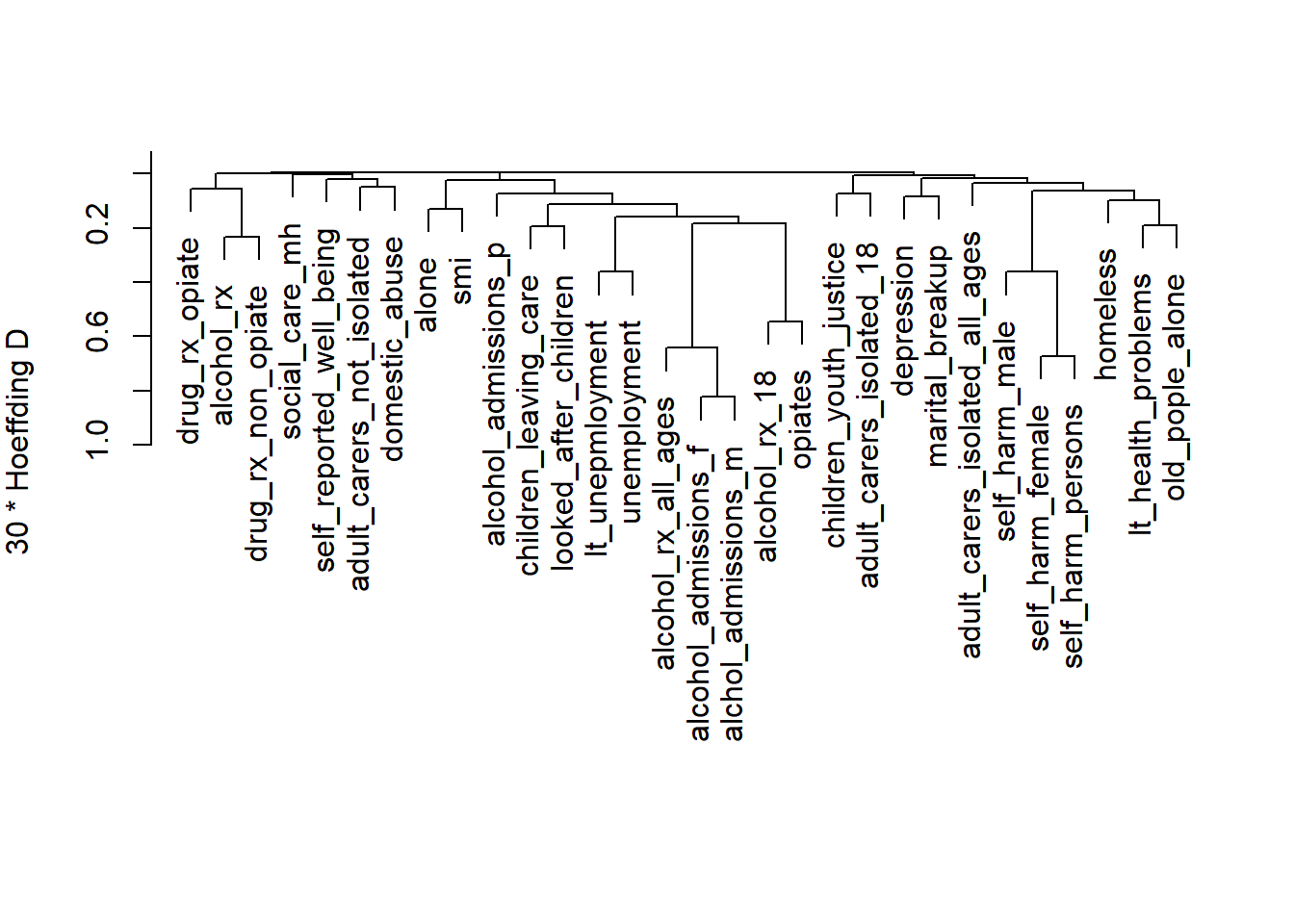
- We can see a lot of the variables clustering together
10.15.3 3. Principal Components Analysis
Let’s examine the data structure using PCA:
# Perform PCA
pca_result <- princomp(df2, cor=TRUE)

# Scree plot
plot(pca_result, type="lines", main="Scree Plot")
abline(h=1, lty=2, col="red")  # Kaiser criterion line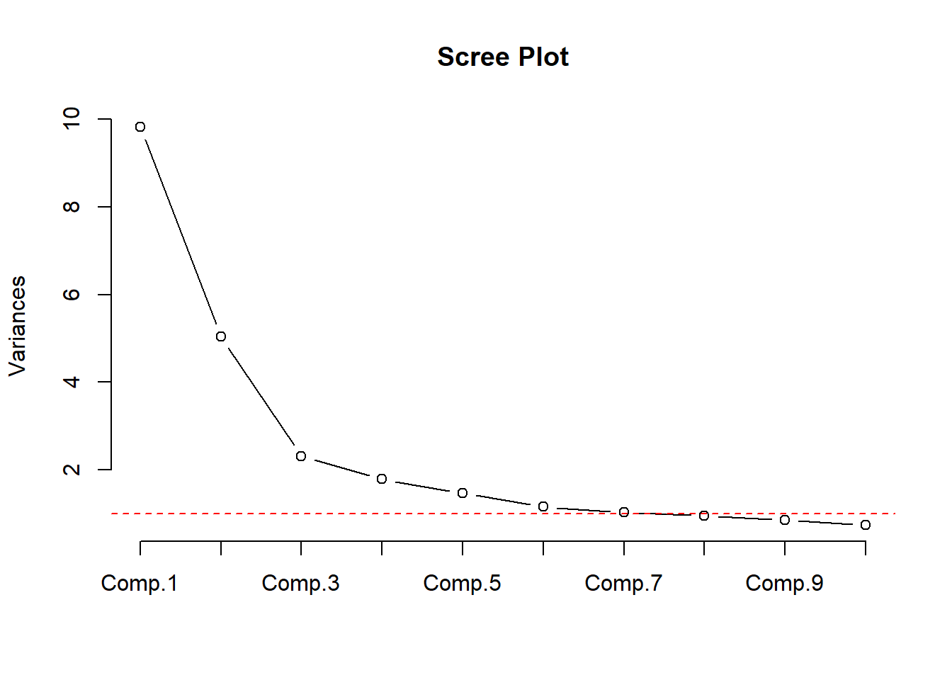
# Print variance explained by first few components
summary(pca_result, loadings=TRUE, cutoff=0.3)
Importance of components:
Comp.1 Comp.2 Comp.3 Comp.4 Comp.5
Standard deviation 3.1327307 2.2436841 1.51857984 1.33713169 1.21224371
Proportion of Variance 0.3271334 0.1678039 0.07686949 0.05959737 0.04898449
Cumulative Proportion 0.3271334 0.4949373 0.57180682 0.63140419 0.68038869
Comp.6 Comp.7 Comp.8 Comp.9 Comp.10
Standard deviation 1.07625280 1.01836888 0.9747646 0.92320127 0.86023787
Proportion of Variance 0.03861067 0.03456917 0.0316722 0.02841002 0.02466697
Cumulative Proportion 0.71899936 0.75356853 0.7852407 0.81365075 0.83831772
Comp.11 Comp.12 Comp.13 Comp.14 Comp.15
Standard deviation 0.76164102 0.74326524 0.70575177 0.67895928 0.65072428
Proportion of Variance 0.01933657 0.01841477 0.01660285 0.01536619 0.01411474
Cumulative Proportion 0.85765429 0.87606907 0.89267192 0.90803811 0.92215284
Comp.16 Comp.17 Comp.18 Comp.19 Comp.20
Standard deviation 0.62502778 0.57314172 0.56636534 0.55357002 0.478567350
Proportion of Variance 0.01302199 0.01094971 0.01069232 0.01021466 0.007634224
Cumulative Proportion 0.93517484 0.94612455 0.95681687 0.96703153 0.974665755
Comp.21 Comp.22 Comp.23 Comp.24
Standard deviation 0.473155304 0.413788556 0.340046283 0.302671397
Proportion of Variance 0.007462531 0.005707366 0.003854382 0.003053666
Cumulative Proportion 0.982128287 0.987835652 0.991690035 0.994743701
Comp.25 Comp.26 Comp.27 Comp.28
Standard deviation 0.250796490 0.224198463 0.174227171 0.1176538993
Proportion of Variance 0.002096629 0.001675498 0.001011837 0.0004614147
Cumulative Proportion 0.996840330 0.998515828 0.999527665 0.9999890799
Comp.29 Comp.30
Standard deviation 1.669952e-02 6.980650e-03
Proportion of Variance 9.295803e-06 1.624316e-06
Cumulative Proportion 9.999984e-01 1.000000e+00
Loadings:
Comp.1 Comp.2 Comp.3 Comp.4 Comp.5 Comp.6 Comp.7
children_youth_justice 0.378 0.580
adult_carers_isolated_18 0.413 0.307
adult_carers_isolated_all_ages
adult_carers_not_isolated
alcohol_rx_18
alcohol_rx_all_ages
alcohol_admissions_f
alchol_admissions_m
alcohol_admissions_p
children_leaving_care
depression
domestic_abuse 0.342
self_harm_female
self_harm_male
self_harm_persons
opiates
lt_health_problems
lt_unepmloyment
looked_after_children
marital_breakup
old_pople_alone 0.338
alone -0.434
self_reported_well_being 0.381
smi -0.366
social_care_mh 0.488
homeless -0.325
alcohol_rx -0.543
drug_rx_non_opiate -0.558
drug_rx_opiate -0.397
unemployment
Comp.8 Comp.9 Comp.10 Comp.11 Comp.12 Comp.13
children_youth_justice
adult_carers_isolated_18
adult_carers_isolated_all_ages 0.351 -0.499 -0.301
adult_carers_not_isolated
alcohol_rx_18
alcohol_rx_all_ages
alcohol_admissions_f
alchol_admissions_m
alcohol_admissions_p -0.378
children_leaving_care
depression 0.340 0.373
domestic_abuse -0.397 0.304
self_harm_female
self_harm_male
self_harm_persons
opiates 0.335
lt_health_problems
lt_unepmloyment
looked_after_children
marital_breakup -0.316 -0.366 0.442
old_pople_alone -0.344
alone
self_reported_well_being 0.605 -0.374
smi
social_care_mh -0.618
homeless
alcohol_rx
drug_rx_non_opiate
drug_rx_opiate 0.312 -0.320
unemployment
Comp.14 Comp.15 Comp.16 Comp.17 Comp.18 Comp.19
children_youth_justice 0.376
adult_carers_isolated_18 -0.505 -0.378
adult_carers_isolated_all_ages 0.304
adult_carers_not_isolated -0.390 0.510 -0.459
alcohol_rx_18
alcohol_rx_all_ages
alcohol_admissions_f
alchol_admissions_m
alcohol_admissions_p 0.376 -0.366
children_leaving_care 0.393
depression -0.304 0.406 -0.387
domestic_abuse 0.311
self_harm_female
self_harm_male
self_harm_persons
opiates -0.305
lt_health_problems
lt_unepmloyment -0.448 -0.334
looked_after_children
marital_breakup
old_pople_alone
alone
self_reported_well_being
smi
social_care_mh
homeless 0.483
alcohol_rx
drug_rx_non_opiate 0.338
drug_rx_opiate -0.382
unemployment
Comp.20 Comp.21 Comp.22 Comp.23 Comp.24 Comp.25
children_youth_justice
adult_carers_isolated_18
adult_carers_isolated_all_ages
adult_carers_not_isolated
alcohol_rx_18
alcohol_rx_all_ages
alcohol_admissions_f
alchol_admissions_m
alcohol_admissions_p
children_leaving_care -0.469
depression
domestic_abuse
self_harm_female 0.495
self_harm_male -0.668
self_harm_persons
opiates
lt_health_problems 0.423
lt_unepmloyment 0.422
looked_after_children 0.634 0.429
marital_breakup -0.370
old_pople_alone 0.307
alone -0.441
self_reported_well_being
smi 0.561 -0.314
social_care_mh
homeless 0.349
alcohol_rx 0.525
drug_rx_non_opiate -0.316 -0.454
drug_rx_opiate
unemployment -0.659
Comp.26 Comp.27 Comp.28 Comp.29 Comp.30
children_youth_justice
adult_carers_isolated_18
adult_carers_isolated_all_ages
adult_carers_not_isolated
alcohol_rx_18 0.342 -0.625
alcohol_rx_all_ages -0.760
alcohol_admissions_f 0.590 0.513
alchol_admissions_m -0.806
alcohol_admissions_p
children_leaving_care
depression
domestic_abuse
self_harm_female 0.487
self_harm_male -0.353 0.338
self_harm_persons -0.804
opiates -0.379 0.435
lt_health_problems 0.479
lt_unepmloyment
looked_after_children
marital_breakup
old_pople_alone -0.488
alone
self_reported_well_being
smi
social_care_mh
homeless
alcohol_rx
drug_rx_non_opiate
drug_rx_opiate
unemployment -0.312 10.15.4 4. Sparse Principal Components Analysis
Using pcaPP for robust sparse PCA.
# Perform sparse PCA
sparse_pca <- sPCAgrid(df2, k=10, method = 'sd' ,
center =mean , scale =sd , scores =TRUE ,
maxiter =10)

# Plot variance explained
plot(sparse_pca,type = 'lines' , main= ' ')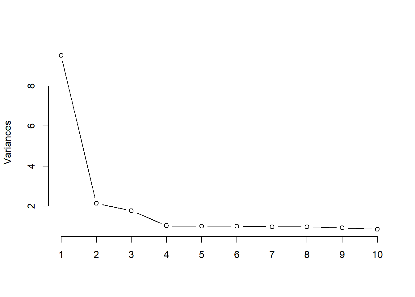
# Print loadings
print(sparse_pca$loadings)
Loadings:
                               Comp.1 Comp.2 Comp.3 Comp.4 Comp.5 Comp.6 Comp.7
children_youth_justice                                             1.000
adult_carers_isolated_18
adult_carers_isolated_all_ages         0.464
adult_carers_not_isolated       0.252
alcohol_rx_18                   0.295
alcohol_rx_all_ages             0.305
alcohol_admissions_f            0.295
alchol_admissions_m             0.303
alcohol_admissions_p            0.161
children_leaving_care           0.248
depression                      0.111
domestic_abuse                  0.106                                     0.791
self_harm_female                0.131               -0.264
self_harm_male                  0.222
self_harm_persons               0.176
opiates                         0.278
lt_health_problems              0.210
lt_unepmloyment                 0.226
looked_after_children           0.300
marital_breakup                 0.113
old_pople_alone                        0.636
alone                           0.122                                    -0.607
self_reported_well_being                             0.965
smi                             0.122
social_care_mh                                              1.000
homeless                              -0.613
alcohol_rx                                    0.707
drug_rx_non_opiate                            0.707
drug_rx_opiate
unemployment                    0.234
                               Comp.8 Comp.9 Comp.10
children_youth_justice
adult_carers_isolated_18
adult_carers_isolated_all_ages
adult_carers_not_isolated
alcohol_rx_18
alcohol_rx_all_ages
alcohol_admissions_f
alchol_admissions_m
alcohol_admissions_p                         -0.574
children_leaving_care
depression                      0.903
domestic_abuse
self_harm_female
self_harm_male
self_harm_persons                      0.444
opiates
lt_health_problems
lt_unepmloyment
looked_after_children
marital_breakup                               0.819
old_pople_alone
alone
self_reported_well_being
smi
social_care_mh
homeless
alcohol_rx
drug_rx_non_opiate
drug_rx_opiate                         0.896
unemployment                   -0.426

               Comp.1 Comp.2 Comp.3 Comp.4 Comp.5 Comp.6 Comp.7 Comp.8 Comp.9
SS loadings     1.000  1.000  1.000  1.000  1.000  1.000  1.000  1.000  1.000
Proportion Var  0.033  0.033  0.033  0.033  0.033  0.033  0.033  0.033  0.033
Cumulative Var  0.033  0.067  0.100  0.133  0.167  0.200  0.233  0.267  0.300
               Comp.10
SS loadings      1.000
Proportion Var   0.033
Cumulative Var   0.333
Like are variable clutstering, we can see that lots of variables load onto the first principal component. We could add component 1 to our regression model and keep the rest of the variables (not those loaded on comp. 1).
However, let’s instead use stepwise regression only on the preditors in combination with sparse PCA to select variables for 10 components in our model.
- Stepwise here tells us which predictors that load onto each PC are needed to predict that pc
spca1 <- princmp(df2, sw = TRUE ,
                 k = 10,
                 kapprox = 10,
                 method = "sparse",
                 cor = TRUE,
                 nvmax = 30)

print(spca1)
Sparse Principal Components Analysis
Stepwise Approximations to PCs With Cumulative R^2
PC 1
alchol_admissions_m (0.975) + self_harm_persons (0.999) +
looked_after_children (1)
PC 2
adult_carers_isolated_all_ages (0.759) + homeless (0.978) +
old_pople_alone (1)
PC 3
drug_rx_non_opiate (0.89) + alcohol_rx (1)
PC 4
self_harm_female (1)
PC 5
adult_carers_isolated_18 (0.861) + self_harm_female (1)
PC 6
self_harm_female (0.993) + self_reported_well_being (1)
PC 7
social_care_mh (1)
PC 8
children_youth_justice (1)
PC 9
domestic_abuse (0.872) + alone (1)
PC 10
depression (0.875) + unemployment (0.999) + old_pople_alone (1)We get 10 components, some with many predictors, some with only one.
10.15.5 Put it all together
Using theory, we could decide to create cluster scores for some of these components, while others with only 2 variables we might want to just eliminate one of the variables.
For those that we want to have a composite score, we can use the first principal component of their scores. Or, if we want to use this scoring outside of this context we can get a regression model on the first PC.
Let me demonstrate with our first component from the sparse PCA.
# Get pc scores for the first sparse PC variables
pc1_scores = princmp(df2[,c(names(spca1$sw[[1]]))],
                     method = "regular",
                     cor = TRUE)$scores[,1]
df2$pc1_scores = pc1_scores

mod1 = lm(pc1_scores~alchol_admissions_m + self_harm_persons , data = df2)

parameters::parameters(mod1) |> print_md()| Parameter | Coefficient | SE | 95% CI | t(146) | p |
|---|---|---|---|---|---|
| (Intercept) | -6.53 | 0.18 | (-6.88, -6.17) | -36.38 | < .001 |
| alchol admissions m | 3.63e-03 | 1.47e-04 | (3.34e-03, 3.92e-03) | 24.70 | < .001 |
| self harm persons | 9.09e-03 | 4.38e-04 | (8.22e-03, 9.95e-03) | 20.75 | < .001 |
Now, we could report those regression coefficients to get a pretty reasonable estimate of the scoring for that component of the model.
Now, let’s get the second and third scores as well.
# Get pc scores for the second sparse PC variables
pc2_scores = princmp(df2[,c(names(spca1$sw[[2]]))],
                     method = "regular",
                     cor = TRUE)$scores[,1]

df2$pc2_scores = pc2_scores

pc3_scores = princmp(df2[,c(names(spca1$sw[[3]]))],
                     method = "regular",
                     cor = TRUE)$scores[,1]

df2$pc3_scores = pc3_scores
For the rest, we will simplify things a bit and just use the first variable of the remaining 10 sparse PCA components.
Let’s now fit a model based using our 3 PCs and the 7 other variables we selected.
df_all = df2 %>%
  select(pc1_scores, pc2_scores, pc3_scores,
         self_harm_female,
         adult_carers_isolated_18,
         self_harm_female,
         social_care_mh,
         children_youth_justice,
         domestic_abuse,
         depression)

df_all$suicide_rate = df$suicide_rate

# 10 predictors, 1 outcome, 149 observations
model_all = lm(
  data = df_all,
  suicide_rate ~ .
)

summary(model_all)
Call:
lm(formula = suicide_rate ~ ., data = df_all)

Residuals:
    Min      1Q  Median      3Q     Max
-4.2067 -1.1131 -0.1051  0.9371  4.1430

Coefficients:
                           Estimate Std. Error t value Pr(>|t|)
(Intercept)               9.6296409  1.6223906   5.935 2.22e-08 ***
pc1_scores                0.5747571  0.1555263   3.696 0.000315 ***
pc2_scores                0.3436984  0.1388871   2.475 0.014539 *
pc3_scores               -0.1009508  0.1084578  -0.931 0.353579
self_harm_female          0.0025597  0.0024544   1.043 0.298819
adult_carers_isolated_18  0.0239721  0.0243409   0.985 0.326408
social_care_mh            0.0010556  0.0004836   2.183 0.030729 *
children_youth_justice   -0.0310969  0.0241586  -1.287 0.200165
domestic_abuse            0.0266173  0.0359734   0.740 0.460599
depression               -0.1202582  0.1114831  -1.079 0.282584
---
Signif. codes:  0 '***' 0.001 '**' 0.01 '*' 0.05 '.' 0.1 ' ' 1

Residual standard error: 1.729 on 139 degrees of freedom
Multiple R-squared:  0.3853,    Adjusted R-squared:  0.3455
F-statistic: 9.681 on 9 and 139 DF,  p-value: 2.122e-11
Now let’s check our assumptions:
check_model(model_all)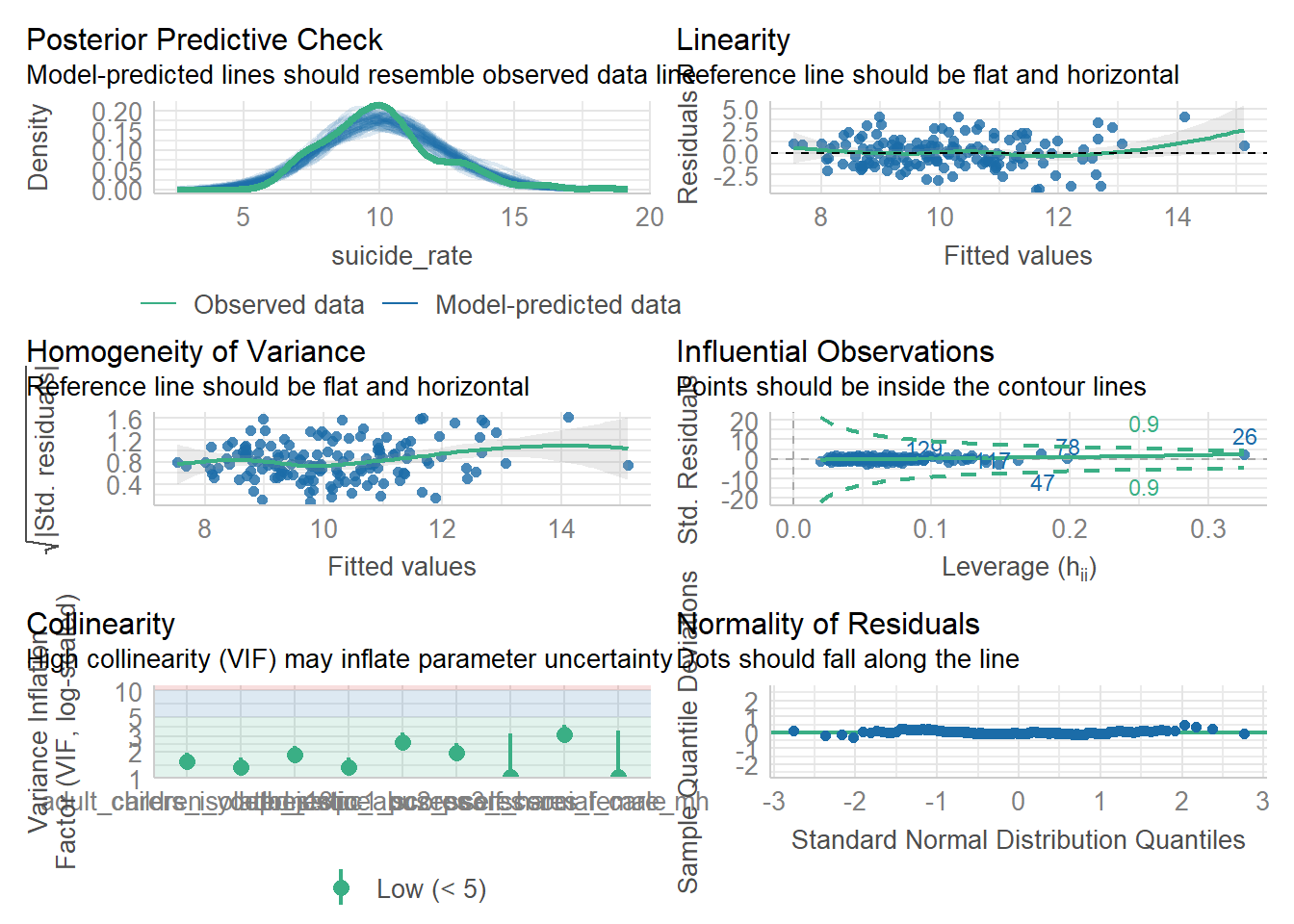
10.15.6 Analysis Summary
From the redundancy analysis, we can identify variables that are highly predictable from others, helping reduce dimensionality while maintaining information.
The variable clustering dendrogram shows natural groupings in our data, which can guide feature selection or creation of composite scores.
The PCA results show how many components are needed to explain a certain percentage of variance in the data.
Sparse PCA provides a more interpretable solution by forcing some loadings to zero while maintaining most of the explained variance.
10.15.7 Recommendations for Data Reduction
Based on these analyses, we can recommend:
Consider combining highly correlated variables within the same cluster into composite scores
Use the first few principal components if dimension reduction is needed while maintaining maximum variance
For interpretability, consider using the sparse PCA solution which provides clearer variable groupings
Remove redundant variables identified in the redundancy analysis on an as needed basis. Justify your choices!
These techniques provide different perspectives on data reduction, and the choice depends on the specific needs of the analysis (interpretability, variance preservation, or prediction accuracy).