2 Data and Models

knitr::opts_chunk$set(echo = FALSE, tidy = TRUE, 
                      cache = FALSE, 
                      message = FALSE, WARNING = FALSE)
# Very standard packages
library(graphics)
library(ggplot2)
library(tidyverse)
library(knitr)
library(readr)
library(MASS)
library(plotly)
library(flextable)
# I do not want default theme.
old.theme <- theme_get()
theme_set(theme_bw())

2.1 Data

2.1.1 Variables and Observations

Let’s talk about what we mean by data, in this course.

Data is composed of variables and observations.

Example: We have a patient. We measure their blood pressure. It is observed to be 133/86.

Variable: Blood pressure

Observation: 133/86

Or we could reformulate this

Variables: Systolic blood pressure and diastolic blood pressure.

Observation(s): 133 and 86

2.1.2 Heart data introduction

heart <- read_csv(here::here("datasets", "Heart.csv"))

as_flextable(head(heart))

age	sex	chestPain	restSysBP	cholesterol	fastBldSgr	restECG	maxHR	exAng	slope	majorVessels	disease
numeric	character	character	numeric	numeric	numeric	numeric	numeric	numeric	numeric	numeric	character
63	Male	typical	145	233	1	2	150	0	3	0	No
67	Male	asymptomatic	160	286	0	2	108	1	2	3	Yes
67	Male	asymptomatic	120	229	0	2	129	1	2	2	Yes
37	Male	nonanginal	130	250	0	0	187	0	3	0	No
41	Female	nontypical	130	204	0	2	172	0	1	0	No
56	Male	nontypical	120	236	0	0	178	0	1	0	No
n: 6

2.1.3 Heart Disease Data Dictionary

A data dictionary explains what the “names” of variables in a dataset mean. For the heart data:

age: The patient’s age in years
sex: The patient’s sex, Male or Female.
chestPain: The chest pain experienced
- typical: typical angina
- nontypical’: abnormal angina
- nonaginal: non-anginal pain
- asymptomatic: no pain
restSysBP: systolic blood pressure upon admission to hospital in mm Hg
cholesterol: The patient’s cholesterol measurement in mg/dl
fastBldSgr: indicator for whether the paitient’s fasting blood sugar was greater than 120 mg/dl: 1 if yes, 0 if no.
restECG: Resting electrocardiographic measurement
- 0: normal
- 1: having ST-T wave abnormality
- 2 showing probable or definite left ventricular hypertrophy by Estes’ criteria
maxHR: The patient’s maximum heart rate achieved during controlled exercise
exAng: Exercise induced angina: 1 if yes, 0 if no
slope: the slope of the peak exercise ST segment
- 1 if slope is positive
- 2 if slope is approximately 0
- 3 if slope is negative
majorVessels: The number of major vessels (0-3) colored in fluoroscopy.
disease: Indicates whether a patient had heart disease: Yes if yes, no if no.

2.2 Mathematical Models

2.2.1 input and output

The whole

The general form of a model is deceptively simple:

\[input \to output.\]

We have some information, the input, we use some process, \(\to\), in order to get some information, the output.

Model: put a quarter in the gumball machine, turn the knob, and a gumball comes out.

Figure 2.1: We have quarter as input to the process, gumball machine, which allows to yield a

2.2.2 Mathematical models

We are doing math here. We will represent our input as \(x\), and our output as \(y\). We put our input \(x\) into some function \(g()\).

\[y = g(x)\]

\(x\) is the input
\(g\) is the \(\to\)
\(y\) is the output

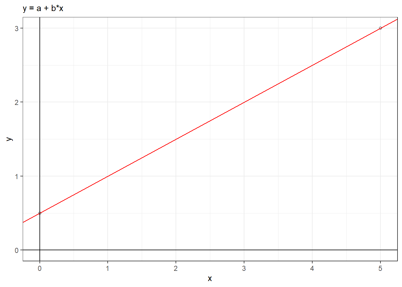
\[ y = a + b \cdot x \]

2.2.3 Heart Model

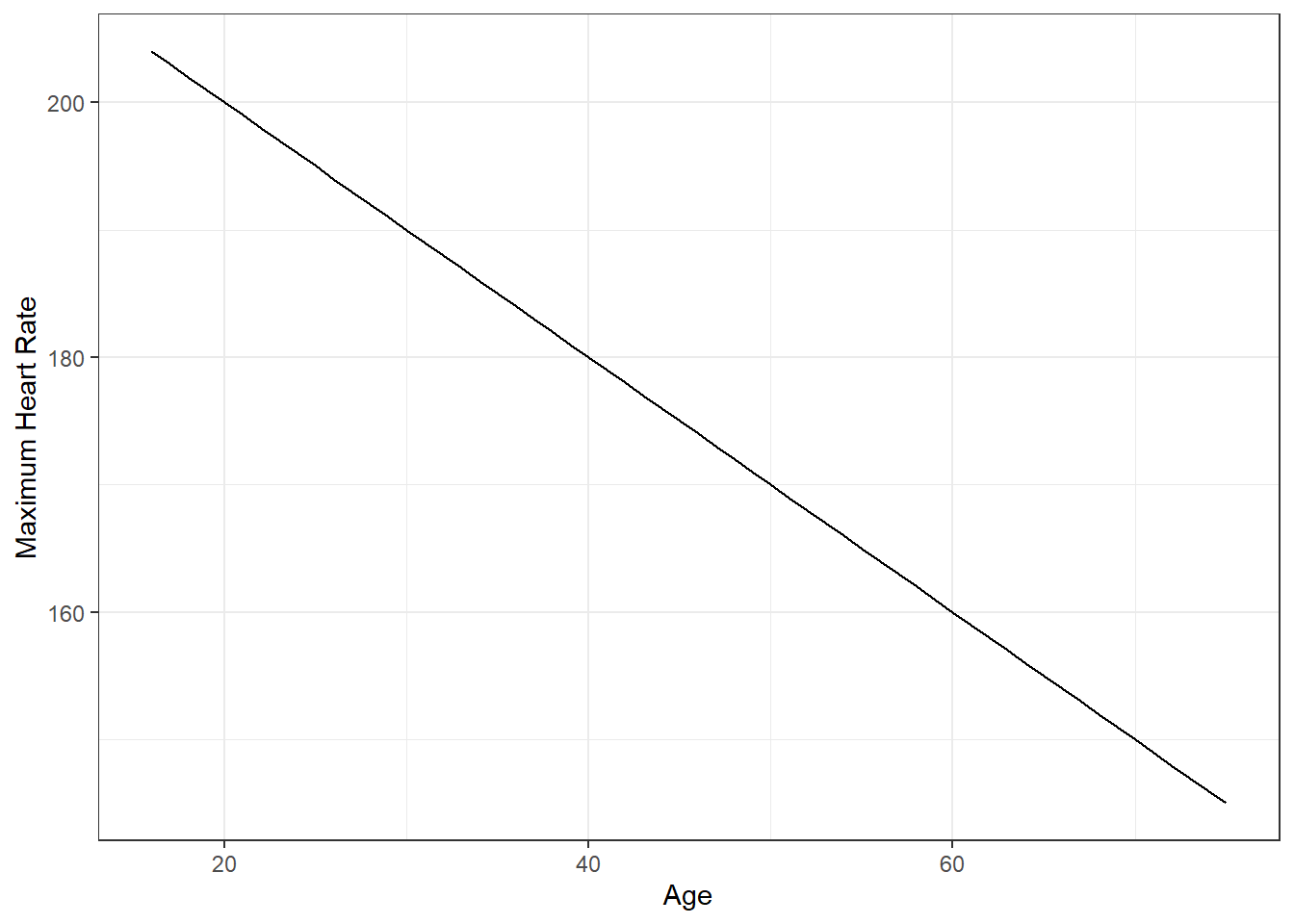
The Mayo Clinic says “You can calculate your maximum heart rate by subtracting your age from 220”.

\(maxHR = 220 - age\)
\(y = 220 - x\)
- y is maxHR
- x is age

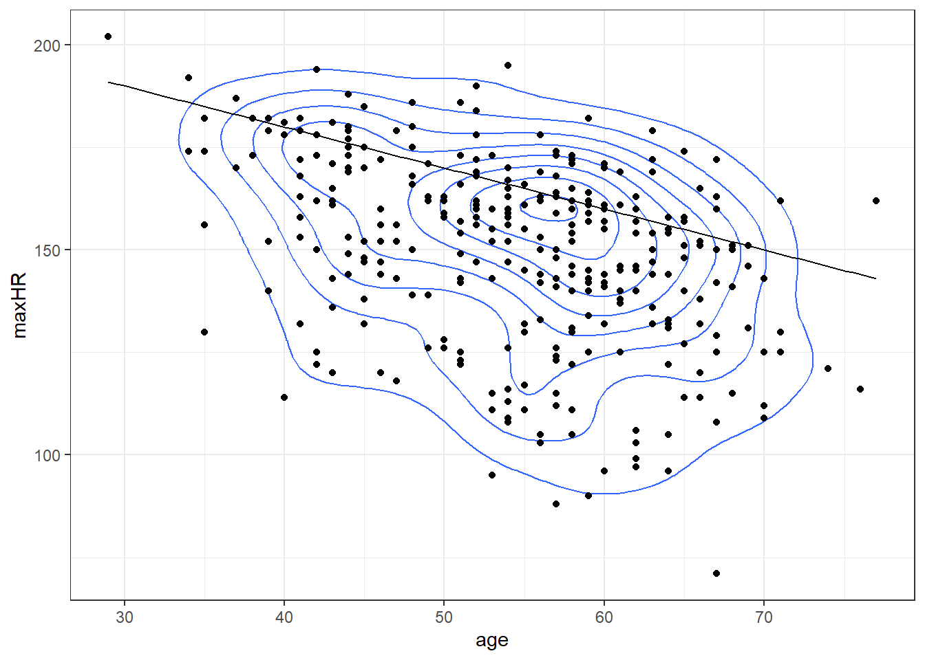
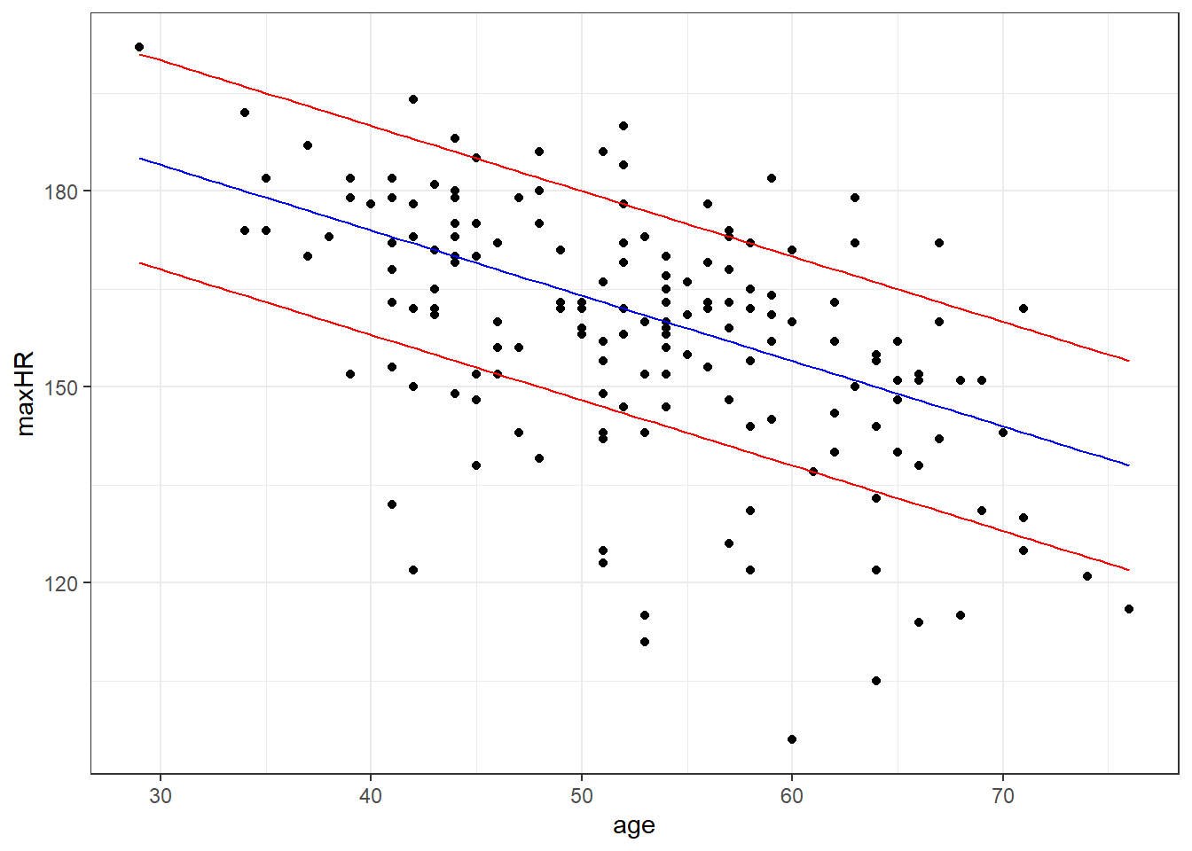
2.2.3.1 What about with the real data?

2.3 Statistical models and Error

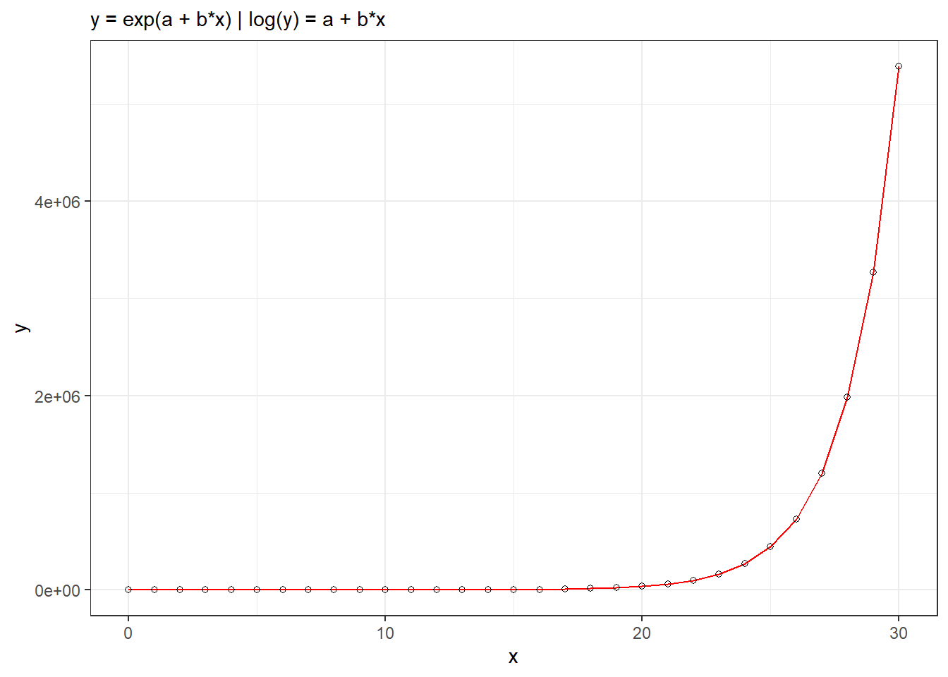
\[y = g(x) + \epsilon\]

y = response
x = predictor
g(x) = function
\(\epsilon\) = error or variability in the model

2.3.1 Heart example

The Mayo Clinic also specifies “You may have a higher or lower maximum heart rate, sometimes by as much as 15 to 20 beats per minute”.

\[MaxHR = 220 - age \pm 20\]

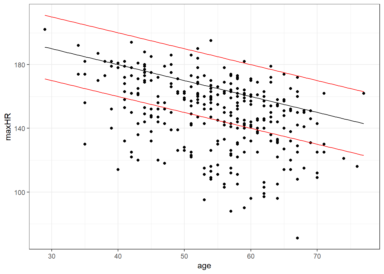
What’s going on here?

The guidelines from the Mayo Clinic apply mainly to the overall population of adults (age 16+).
This data is based on a study about heart disease.
Primarily, there are two groups in the data: those with heart disease, and those without.
Maybe heart disease has an effect.

2.3.1.1 Grouping Means

2.3.2 Conditional Means vs Unconditional Means

Let’s concentrate on the formula for basic statistical models.

\[y = g(x) + \epsilon\]

2.3.2.1 Simplest Example

Unconditional Mean

\[y = \mu + \epsilon\]

2.3.2.2 Simple Model With Disease

\[y = 140 \pm 23\] Why might we use this model?

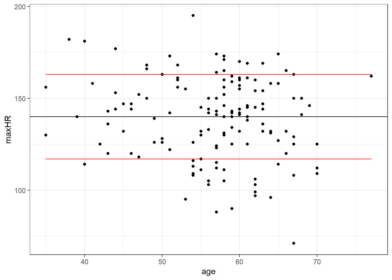
Percent 140 +/- 23
82.01439

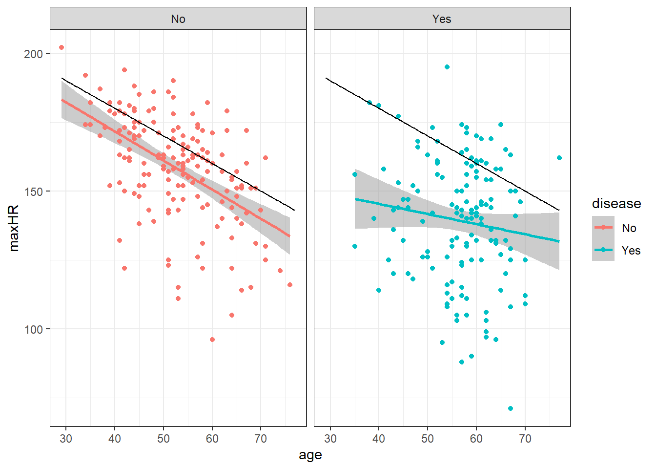
2.3.2.3 Model for Those Without Disease

The average maxHR should be about 214 - age, the standard deviation of that model is about 16

We denote this as:

\[y = 214 - x \pm 16\]

Percent 214 - x +/- 16
0.7256098

2.4 Linear models

2.4.1 Simple linear models: one predictor variable.

The simple linear model says the \(\mu_{y|x}\) is a line that depends on \(x\) based on a \(y\)-intercept which we denote by \(\beta_0\) and a slope which we denote \(\beta_1\).

\[\mu_{y|x} = \beta_0 + \beta_1 x\]

Conditional mean (deterministic)
\(\beta_0\): y-intercept
\(\beta_1\): slope

\[ y = \beta_0 + \beta_1 x + \epsilon = \mu_{y|x} + \epsilon \]

\(\epsilon\) is the error in the model (noted as “randomness” in some lecture videos¹)

2.4.2 Linear models with more than one predictor variable

A linear model in general means a model that can be written as a sum of variables and coefficients:

\[y = \beta_0 + \sum_{i=1}^k\beta_i x_i + \epsilon\]

\(\mu_{y | x}\) deterministic
\(\epsilon\) is the model error

\[ y = \beta_0 + \beta_1x_1 + \beta_2x_2 + \beta_3x_3 + ... + \beta_kx_k + \epsilon \]

We should ↩︎