# Here are the libraries I used
library(tidyverse) # standard
library(knitr) # need for a couple things to make knitted document to look nice
library(readr) # need to read in data
library(ggpubr) # allows for stat_cor in ggplots
library(ggfortify) # Needed for autoplot to work on lm()
library(gridExtra) # allows me to organize the graphs in a grid7 Transformations
Here are some code chunks that setup this chapter.
# This changes the default theme of ggplot
old.theme <- theme_get()
theme_set(theme_bw())
Again our model is
\[y = \beta_0 + \beta_1 x + \epsilon\]
where \(\epsilon \sim N(0,\sigma).\)
\[ x \rightarrow g(x) \]
\[ h(y)= \beta_0 + \beta_1g(x) + \epsilon \]
\[ y \rightarrow h(y) \]
7.1 Not all relations are linear
You’ll have to forgive me for a non-biostatistics example, but it exemplifies what I want to discuss in a simple and easily understandable way (I think).
We’re going to take a look at some cars.
cars <- read_csv(here::here("datasets",
                            'cars04.csv'))
Rows: 428 Columns: 14
── Column specification ────────────────────────────────────────────────────────
Delimiter: ","
chr (3): Name, Type, Drive
dbl (11): MSRP, Dealer, Engine, Cyl, HP, CMPG, HMPG, Weight, WheelBase, Leng...
ℹ Use `spec()` to retrieve the full column specification for this data.
ℹ Specify the column types or set `show_col_types = FALSE` to quiet this message.Several variables to examine, but we’ll just parse it down to looking at the relation between the Weight of vehicles and their fuel efficiency in terms of Miles Per Gallon (MPG). CMPG is the typical MPG in a city environment, and HMPG is the tyical MPG on highways/interstates/non-stop-and-go driving.
7.1.1 Correlations
# I am using arguments in the second stat_cor to change the location of the text
# This is so that the two correlations don't overlap.
ggplot(cars, aes(x = Weight, y = CMPG)) +
  geom_point() +
  geom_smooth(method = "lm", formula = y~x) +
  stat_cor(method = "pearson") +
  stat_cor(method = "kendall", label.y = 55, color = "blue")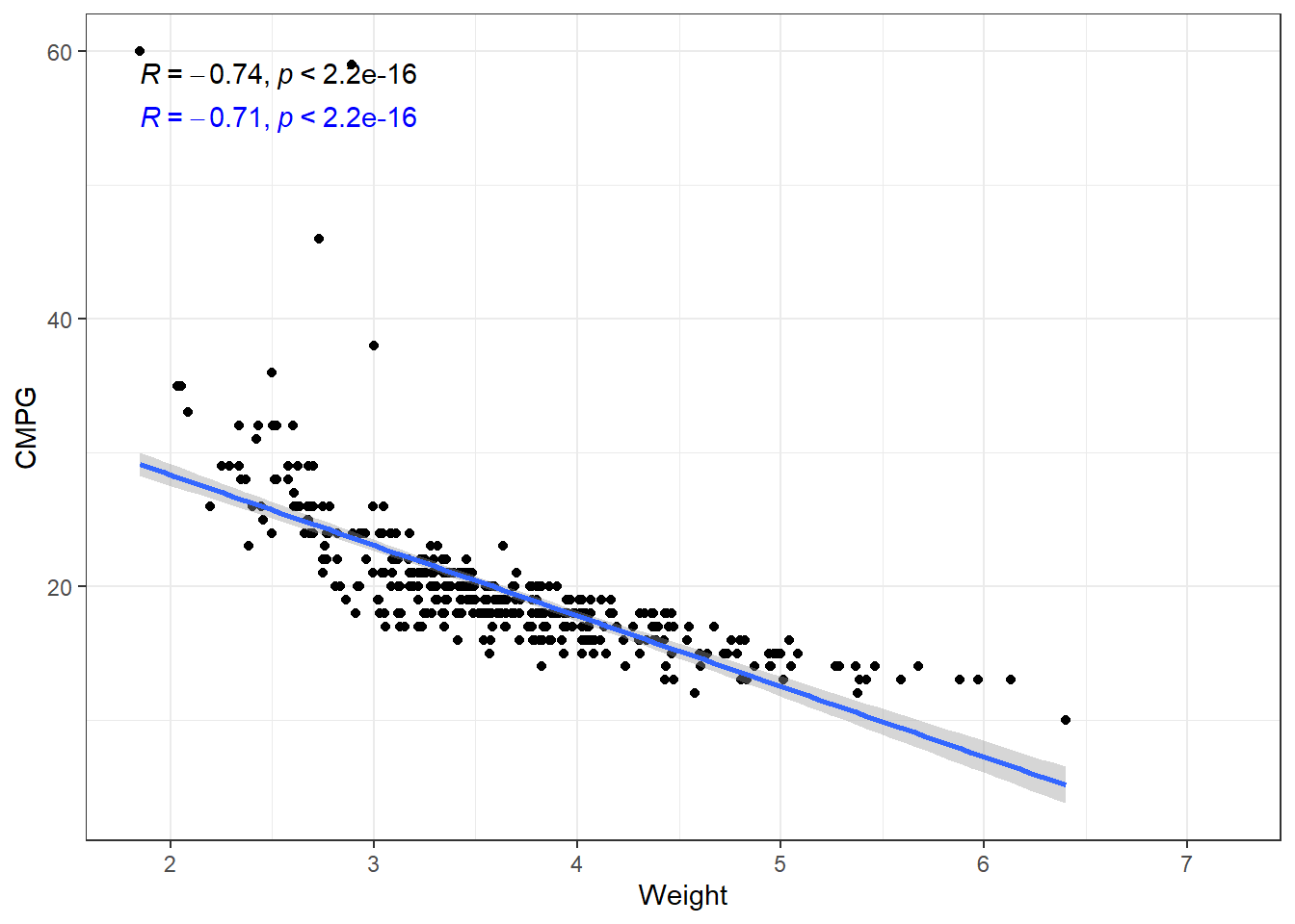
The relation is fairly strong, but does not appear linear. There seems to be a curve to it. The linear model plotted is biased. This means that at some points we expect values to fall below the line more often than not. And other places, we expect the values to fall above the line.
7.1.2 Residuals
This would be reflected residual diagnostics.
carsLm <- lm(CMPG ~ Weight, cars)
autoplot(carsLm)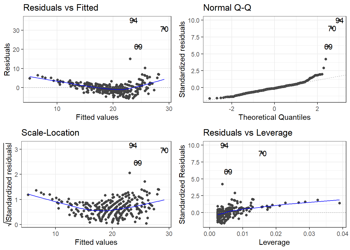
Typically we want to force the data into a linear pattern.
7.1.3 Transformations for Non-linear Relationships
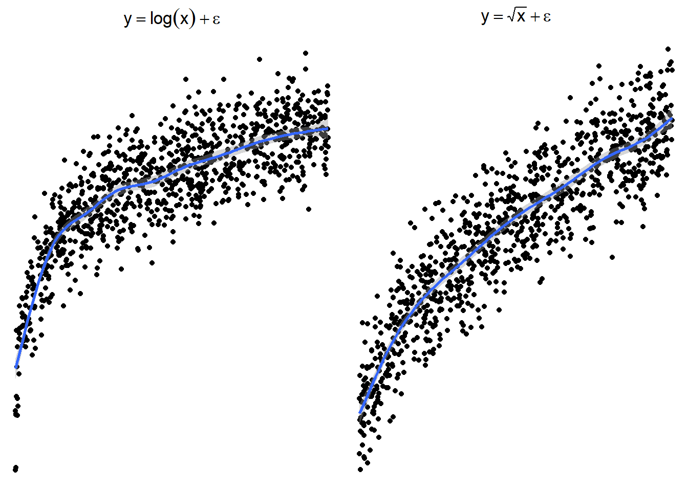
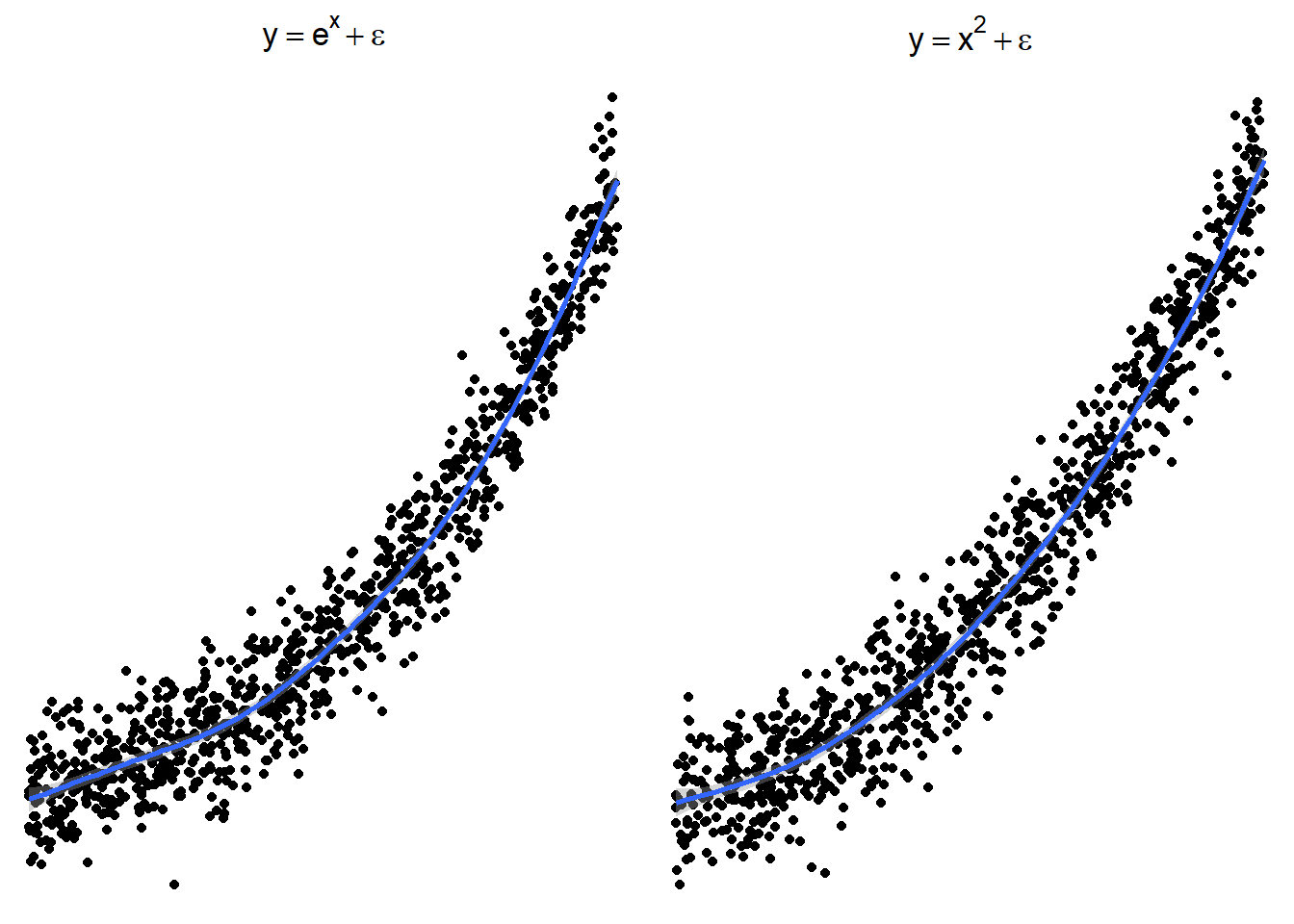
The following plots show several non-linear relationships. With each scatterplot there is the correct transformation for the \(x\) variable.
7.1.3.1 \(\log(x)\) and \(\sqrt x\)
7.1.3.2 \(x^2\) or \(e^x\) (sometimes \(e^x\) is denoted by \(\exp(x)\))
7.1.3.3 \(1/x\) or \(e^{-x}\) (or \(\exp(-x)\))
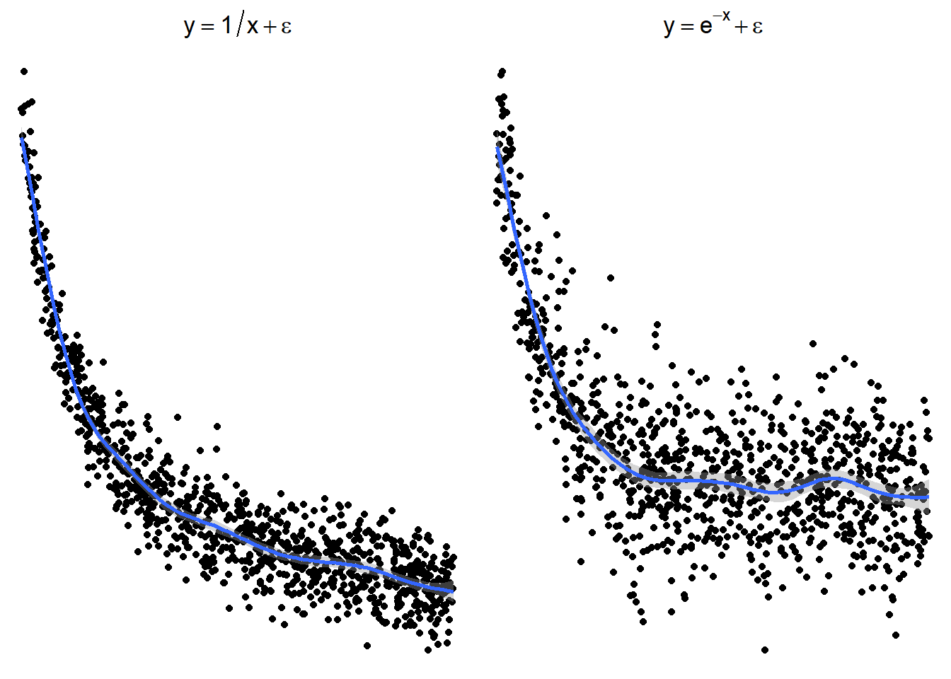
These are just guidelines for which transformations may help. Sometimes the transformations the other transformations may be appropriate because the relationship is flipped by a negative sign.
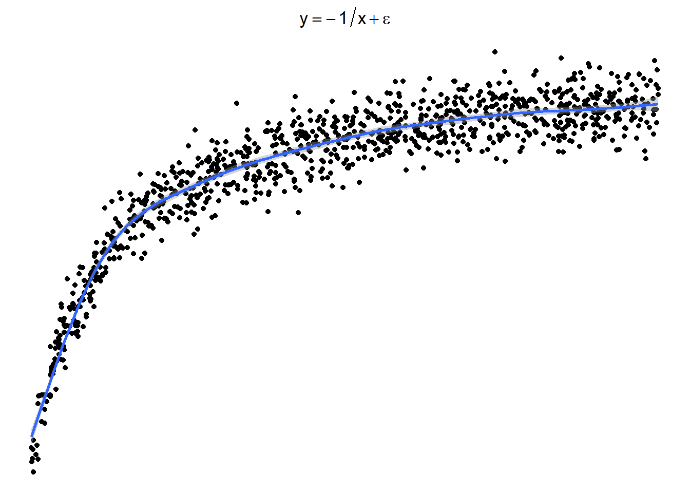
7.1.3.4 Sometimes things look one way and are another
Here is a graph of the model \(y = -\frac{1}{x} + \epsilon\)
7.1.3.5 Trying \(\log(x)\) or \(\sqrt x\)
Here are side by side graphs of the original data and transforming the \(x\) variable using \(\log(x)\), \(\sqrt x\), and \(1/x\).
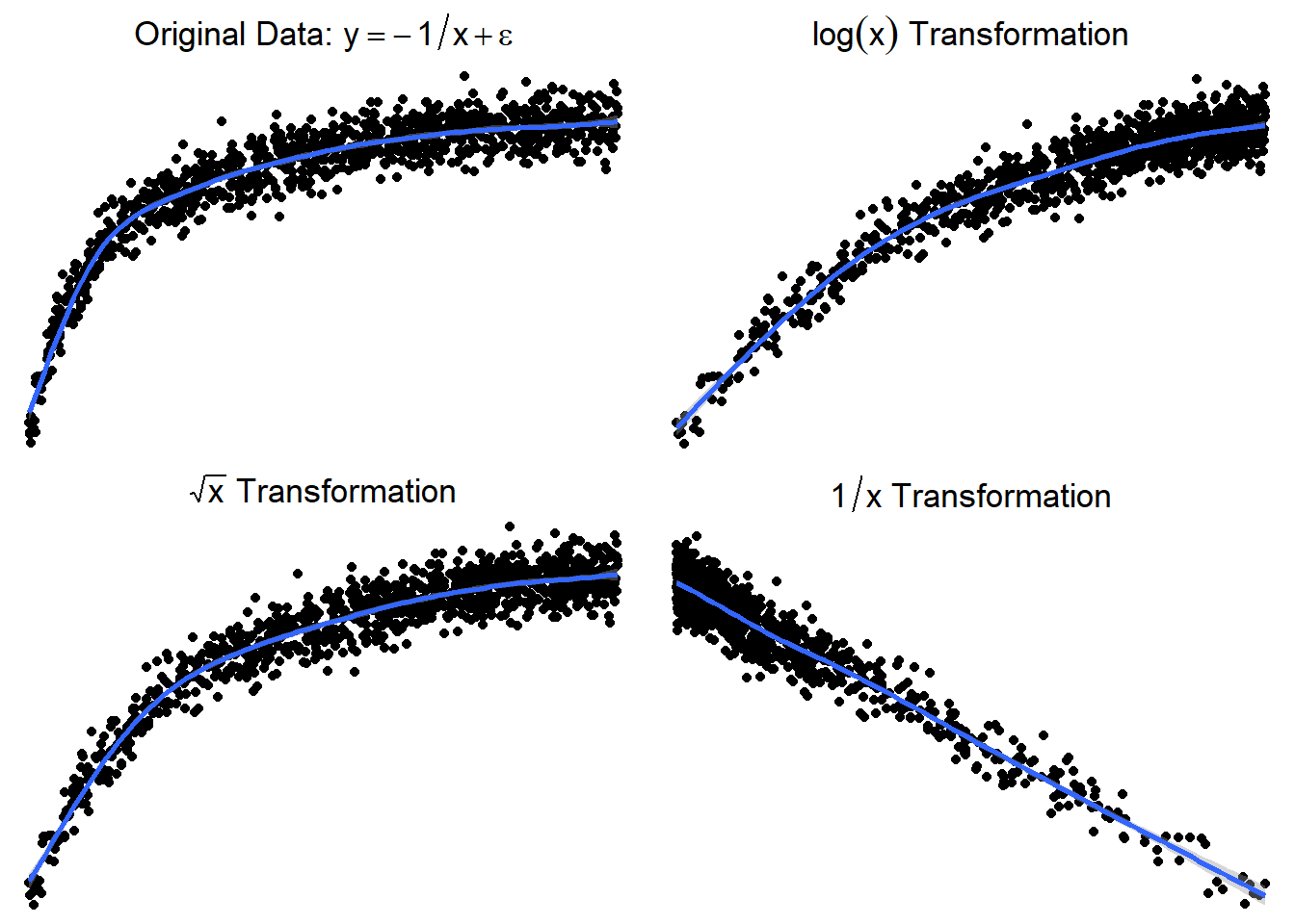
It is important that you try several transformations before giving up on a linear regression model.
7.1.4 Applying a transformation to the cars dataset
p1 <- ggplot(cars, aes(x = Weight, y = CMPG)) +
  geom_point() +
  geom_smooth(method = "lm")

p2 <- ggplot(cars, aes(x = 1/Weight, y = CMPG)) +
  geom_point() +
  geom_smooth(method = "lm")

grid.arrange(p1,p2, nrow = 1)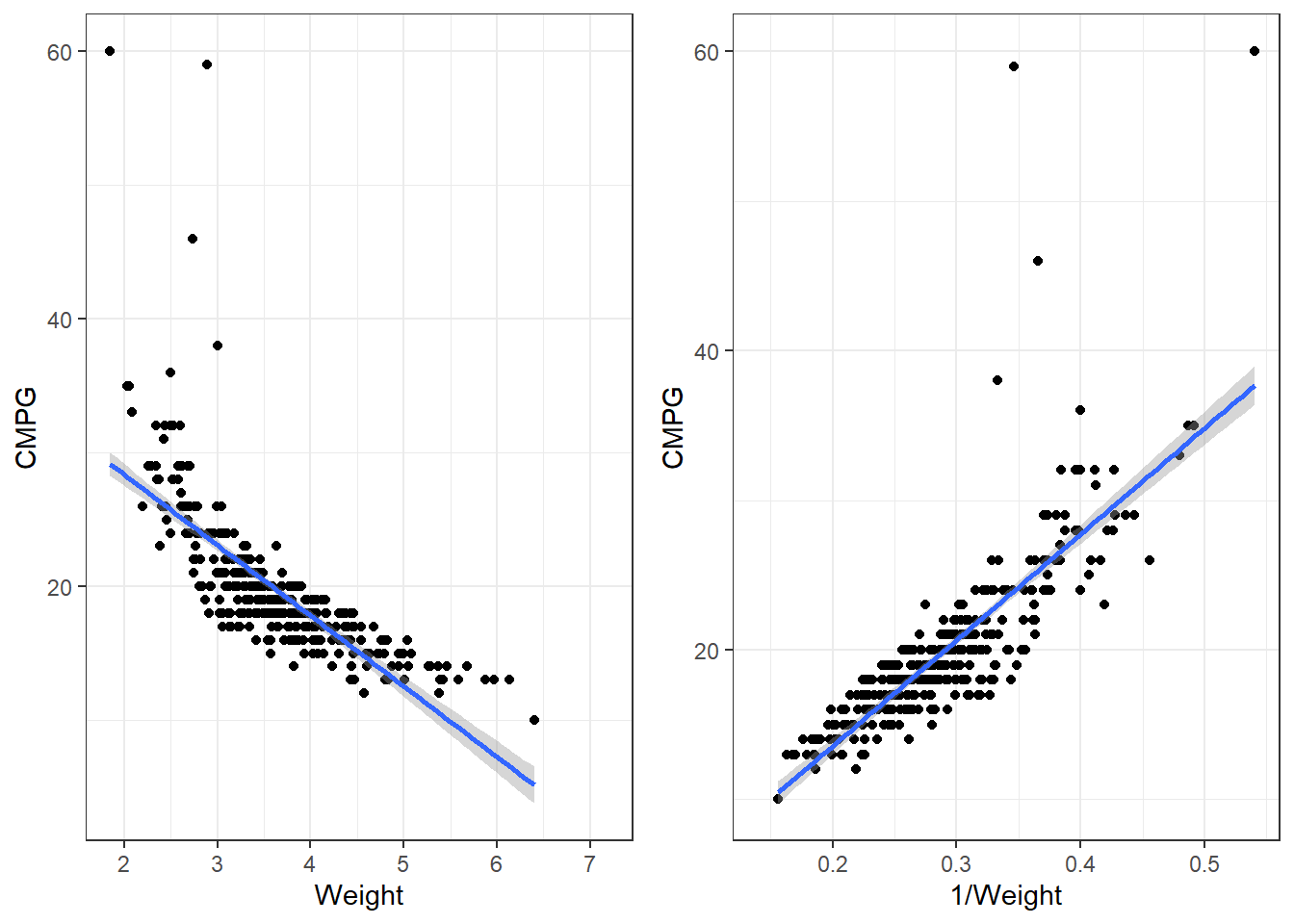
7.1.4.1 Transformations in lm()
When performing transformation in linear models, those can be done within the lm() function. Instead of lm(y ~ x, data), you can put lm(y ~ I(g(x)), data).
g(x)is whatever transformation on the \(x\) variable you are trying.I()is anRsyntax thing that is needed sometimes so that the functiong(x)is interpreted correctly.Though
I()is not always necessary, it is best practice to use it every time you re performing a transformation.
Our function is 1/Weight, so we would write for the formula, y ~ I(1/Weight). In this case, is is necessary to use I(). Try summarising a model where the formula is
carsLm2 <- lm(CMPG ~ I(1/Weight), cars)
summary(carsLm2)
Call:
lm(formula = CMPG ~ I(1/Weight), data = cars)

Residuals:
   Min     1Q Median     3Q    Max
-6.088 -1.302  0.069  1.040 35.073

Coefficients:
            Estimate Std. Error t value Pr(>|t|)
(Intercept)  -0.5651     0.7629  -0.741    0.459
I(1/Weight)  70.7812     2.5606  27.642   <2e-16 ***
---
Signif. codes:  0 '***' 0.001 '**' 0.01 '*' 0.05 '.' 0.1 ' ' 1

Residual standard error: 3.09 on 410 degrees of freedom
  (16 observations deleted due to missingness)
Multiple R-squared:  0.6508,    Adjusted R-squared:  0.6499
F-statistic: 764.1 on 1 and 410 DF,  p-value: < 2.2e-16
7.1.4.2 Residuals
autoplot(carsLm2)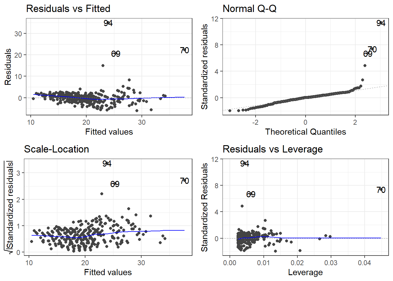
7.2 “Stabilizing” Variability
Sometimes the standard deviation of the residuals is constant on a relative scale.
\[CV = \frac{\sigma_\epsilon}{|\mu_{y|x}|}\] The \(\log\) is typical the transformation used in this situation.
\[\log(y) = \beta_0 + \beta_1 x + \epsilon \qquad \iff \qquad y = e^{\beta_0 + \beta_1 x +\epsilon}\]
Other possibilities would be taking the square root (or higher power root) of the \(y\) variable, but most often it is \(\log\) that works best if a \(y\) transformation is viable.
7.2.1 Log of cars data
There are many potential models. We have to account for non-linearity and the variability issue.
p1 <- ggplot(cars, aes(x = Weight, y = CMPG)) +
  geom_point() +
  geom_smooth() +
  labs(title = expression(paste("No Transformation"))) #expression() lets me show math

p2 <- ggplot(cars, aes(x = Weight, y = log(CMPG))) +
  geom_point() +
  geom_smooth() +
  labs(title = expression(paste(log(y), " Transformation"))) #expression() lets me show math

p3 <- ggplot(cars, aes(x = 1/Weight, y = CMPG)) +
  geom_point() +
  geom_smooth() +
  labs(title = expression(paste(1/x, " Transformation"))) #expression() lets me show math

p4 <- ggplot(cars, aes(x = 1/Weight, y = log(CMPG))) +
  geom_point() +
  geom_smooth() +
labs(title = expression(paste(log(y), " and ", 1/x, "Transformations"))) #expression() lets me show mathgrid.arrange(p1,p2,p3,p4)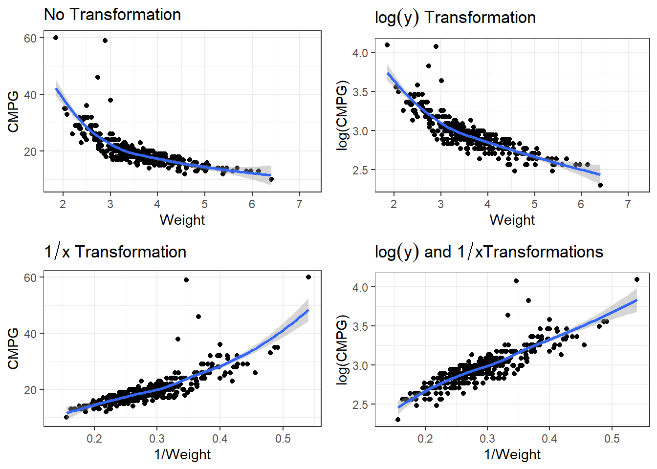
7.2.1.1 Linear Model
carsLm3 <- lm(log(CMPG) ~ I(1/(Weight)), data = cars)

summary(carsLm3)
Call:
lm(formula = log(CMPG) ~ I(1/(Weight)), data = cars)

Residuals:
     Min       1Q   Median       3Q      Max
-0.25328 -0.05547  0.00506  0.05825  0.92912

Coefficients:
              Estimate Std. Error t value Pr(>|t|)
(Intercept)    2.03375    0.02710   75.06   <2e-16 ***
I(1/(Weight))  3.22138    0.09094   35.42   <2e-16 ***
---
Signif. codes:  0 '***' 0.001 '**' 0.01 '*' 0.05 '.' 0.1 ' ' 1

Residual standard error: 0.1098 on 410 degrees of freedom
  (16 observations deleted due to missingness)
Multiple R-squared:  0.7537,    Adjusted R-squared:  0.7531
F-statistic:  1255 on 1 and 410 DF,  p-value: < 2.2e-16
carsLm3 <- lm(log(CMPG) ~ I(1/(Weight)), data = cars)
summary(carsLm3)
Call:
lm(formula = log(CMPG) ~ I(1/(Weight)), data = cars)

Residuals:
     Min       1Q   Median       3Q      Max
-0.25328 -0.05547  0.00506  0.05825  0.92912

Coefficients:
              Estimate Std. Error t value Pr(>|t|)
(Intercept)    2.03375    0.02710   75.06   <2e-16 ***
I(1/(Weight))  3.22138    0.09094   35.42   <2e-16 ***
---
Signif. codes:  0 '***' 0.001 '**' 0.01 '*' 0.05 '.' 0.1 ' ' 1

Residual standard error: 0.1098 on 410 degrees of freedom
  (16 observations deleted due to missingness)
Multiple R-squared:  0.7537,    Adjusted R-squared:  0.7531
F-statistic:  1255 on 1 and 410 DF,  p-value: < 2.2e-16
So \[\widehat{\log(CMPG)} = 2.03 + 3.22\frac{1}{Weight}\] is our estimated regression line.
7.2.1.2 Residuals
autoplot(carsLm3)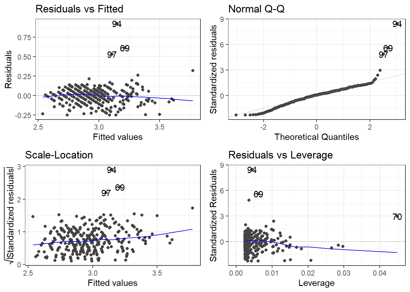
7.2.1.3 Outliers
outliers <- c(94, 69, 97, 70)

cars[outliers, ]
# A tibble: 4 × 14
Name Type Drive MSRP Dealer Engine Cyl HP CMPG HMPG Weight WheelBase
<chr> <chr> <chr> <dbl> <dbl> <dbl> <dbl> <dbl> <dbl> <dbl> <dbl> <dbl>
1 Toyo… Car FWD 20510 18926 1.5 4 110 59 51 2.89 106
2 Hond… Car FWD 20140 18451 1.4 4 93 46 51 2.73 103
3 Volk… Car FWD 21055 19638 1.9 4 100 38 46 3.00 99
4 Hond… Car FWD 19110 17911 2 3 73 60 66 1.85 95
# ℹ 2 more variables: Length <dbl>, Width <dbl>filter(cars, Weight < 2.1)# A tibble: 4 × 14
Name Type Drive MSRP Dealer Engine Cyl HP CMPG HMPG Weight WheelBase
<chr> <chr> <chr> <dbl> <dbl> <dbl> <dbl> <dbl> <dbl> <dbl> <dbl> <dbl>
1 Toyo… Car FWD 10760 10144 1.5 4 108 35 43 2.04 93
2 Toyo… Car FWD 11560 10896 1.5 4 108 33 39 2.08 93
3 Toyo… Car FWD 11290 10642 1.5 4 108 35 43 2.06 93
4 Hond… Car FWD 19110 17911 2 3 73 60 66 1.85 95
# ℹ 2 more variables: Length <dbl>, Width <dbl>removeOutliers <- c(94, 69, 70)
cars2 <- cars[-removeOutliers, ]7.2.1.4 Removing outliers and new model
carsLm4 <- lm(log(CMPG) ~ I(1/Weight), cars2)

summary(carsLm4)
Call:
lm(formula = log(CMPG) ~ I(1/Weight), data = cars2)

Residuals:
     Min       1Q   Median       3Q      Max
-0.25752 -0.05228  0.00710  0.05943  0.54103

Coefficients:
            Estimate Std. Error t value Pr(>|t|)
(Intercept)  2.06635    0.02359   87.60   <2e-16 ***
I(1/Weight)  3.09371    0.07948   38.92   <2e-16 ***
---
Signif. codes:  0 '***' 0.001 '**' 0.01 '*' 0.05 '.' 0.1 ' ' 1

Residual standard error: 0.09357 on 407 degrees of freedom
  (16 observations deleted due to missingness)
Multiple R-squared:  0.7882,    Adjusted R-squared:  0.7877
F-statistic:  1515 on 1 and 407 DF,  p-value: < 2.2e-16
Compare to model with outliers.
7.2.1.5 Checking residuals AGAIN
autoplot(carsLm4)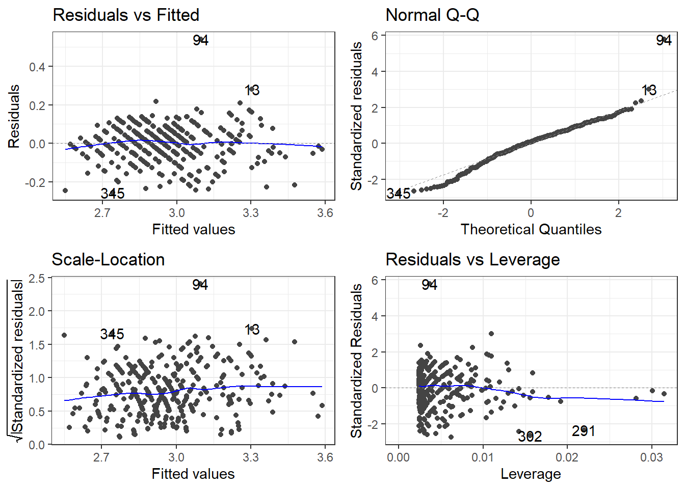
7.3 You’ve got a linear model, now what
\[\widehat{\log(CMPG)} = 2.03 + 3.22\frac{1}{Weight} \qquad \iff \qquad \widehat{CMPG} = e^{2.03 + 3.22\frac{1}{Weight}} \]
7.3.1 Interpreting you coefficients
We’ve got this model. How would we explain what it says?
\[\widehat{\log(CMPG)} = 2.03 + 3.22\frac{1}{Weight}\]
This means we are looking at how \(1/Weight\) affects the relative change of \(CMPG\). What does that mean?
Say you were to look at the average weight of cars that weighed \(d\) thousand pounds more. The change in log of CMPG is
\[\Delta \log(CMPG) = \frac{3.22}{Weight + d} - \frac{3.22}{Weight} = \frac{-3.22d}{Weight^2 + d\cdot Weight}\]
Using math “magic”.
\[CMPG_d = CMPG_0 \cdot e^{\frac{-3.22d}{Weight^2 + d\cdot Weight}}\]
In terms of viewing the model as \(\widehat{CMPG} = e^{2.03 + 3.22\frac{1}{Weight}}\) the change in \(CMPG\) would be
\[\Delta \widehat{CMPG} = \left(e^{2.03 + 3.22\frac{1}{Weight}}\right) - \left(e^{2.03 + 3.22\frac{1}{Weight + d}}\right)\]
I don’t know about this form either.
7.3.2 Predictions from transformations
You create a data.frame that contains the values of the predictor variable that you want predictions for, and then plug them into the predict() function.
newdata <- data.frame(Weight = c(1.5, 2, 2.5, 3, 3.5, 4))

predictions <- predict(carsLm4, newdata)
Now let’s look at those predictions.
predictions 1 2 3 4 5 6
4.128824 3.613205 3.303834 3.097587 2.950267 2.839777 There’s an issue here. These are the predictions for \(\log(CMPG)\), not CMPG. You have to use the reverse function on the predictions. In this case, log(y) takes the natural log of \(y\). Therefore, your reverse function is \(e^y\) using exp(y).
exp(predictions) 1 2 3 4 5 6
62.10485 37.08473 27.21679 22.14445 19.11106 17.11196 7.3.2.1 Confidence and Interval Intervals
Likewise, if you wanted confidence intervals for the mean, or prediction intervals for future observations, you would specify an interval = "confidence" or interval = "prediction" argument and a level argument specifying the desired confidence level for your intervals. AND you need to apply the reverse function.
CIs <- predict(carsLm4, newdata, interval = "confidence", level = 0.99)

PIs <- predict(carsLm4, newdata, interval = "prediction", level = 0.99)
Here are the 99% confidence intervals.
exp(CIs) fit lwr upr
1 62.10485 57.43392 67.15565
2 37.08473 35.46636 38.77696
3 27.21679 26.53386 27.91730
4 22.14445 21.81908 22.47467
5 19.11106 18.88265 19.34223
6 17.11196 16.86310 17.36448And here are the 99% prediction intervals.
exp(PIs) fit lwr upr
1 62.10485 48.15157 80.10149
2 37.08473 28.99050 47.43889
3 27.21679 21.33490 34.72030
4 22.14445 17.37399 28.22475
5 19.11106 14.99637 24.35473
6 17.11196 13.42575 21.81026Confidence levels when you apply the reverse transformations are only approximate. Actual confidence may be higher or lower. Something about this thing called Jensen’s inequality…