Hypothesis Testing with TOSTER

Introduction

TOSTER was originally conceived as an equivalence testing package, but it is really a general-purpose hypothesis testing toolkit. Equivalence testing via the two one-sided tests (TOST) procedure is one of its core features, but the package also supports standard null hypothesis significance tests, non-inferiority testing, and superiority-by-a-margin testing through a single, consistent interface.

Many of TOSTER’s test functions return objects of class htest, the same structure used by base R functions like t.test(), wilcox.test(), and cor.test(). This means results from TOSTER plug directly into existing R workflows. On top of this, TOSTER provides helper functions for tabulating, describing, and plotting test results that work with most htest objects.

The central idea is simple: hypothesis testing involves specifying a null hypothesis, choosing an alternative, and evaluating by a test. By adjusting the alternative and mu (or null depending on the function) arguments in TOSTER’s functions, you can move seamlessly between testing frameworks. A standard nil-hypothesis test, an equivalence test, a non-inferiority analysis, and a superiority-by-a-margin test are all handled by the same interface.

library(TOSTER)

Throughout this vignette we use the built-in sleep dataset, which contains extra hours of sleep (extra) for 10 subjects under two drug conditions (group).

The simple_htest Interface

simple_htest() is a unified wrapper for common two-group (and one-sample) hypothesis tests. It calls base R’s t.test() or wilcox.test() under the hood but improves the output in two ways:

1. Sample sizes are reported are saved in the output (base R does not record n).
2. The effect is shown explicitly as a difference (e.g., “mean difference (1 - 2)”) rather than listing two group means and leaving the reader to compute the difference.

Basic usage: two-sample t-test

A standard two-sided t-test with simple_htest looks just like t.test() but with a formula interface and explicit mu argument:

test1 = simple_htest(extra ~ group,
             data = sleep,
             mu = 0,
             alternative = "two.sided")

test1$sample_size
#>  1  2 
#> 10 10

Compare this with base R’s t.test():

t.test(extra ~ group, data = sleep)
#> 
#>  Welch Two Sample t-test
#> 
#> data:  extra by group
#> t = -1.8608, df = 17.776, p-value = 0.07939
#> alternative hypothesis: true difference in means between group 1 and group 2 is not equal to 0
#> 95 percent confidence interval:
#>  -3.3654832  0.2054832
#> sample estimates:
#> mean in group 1 mean in group 2 
#>            0.75            2.33

Notice that simple_htest saves the sample sizes in each group and appends the mean difference to the output, saving the reader a calculation step. Additionally, notice how group labels are applied so you don’t have to guess which group mean was sbutracted from which (i.e., mean difference ('1' - '2')).

Wilcoxon test

To run a nonparametric Wilcoxon rank-sum test instead of a t-test, set the test argument:

simple_htest(extra ~ group,
             data = sleep,
             test = "wilcox.test",
             mu = 0,
             alternative = "two.sided")
#> Warning in wilcox.test.default(x = x, y = y, paired = paired, conf.int = TRUE,
#> : cannot compute exact p-value with ties
#> Warning in wilcox.test.default(x = x, y = y, paired = paired, conf.int = TRUE,
#> : cannot compute exact confidence intervals with ties
#> 
#>  Wilcoxon rank sum test with continuity correction
#> 
#> data:  extra by group
#> W = 25.5, p-value = 0.06933
#> alternative hypothesis: true location shift is not equal to 0
#> 95 percent confidence interval:
#>  -3.59994709  0.09995356
#> sample estimates:
#> Hodges-Lehmann estimate ('1' - '2') 
#>                           -1.346388

The output includes the Hodges-Lehmann estimate of the location shift. Please note that this estimate is not a the mean or median difference, but rather the median of all pairwise differences between groups (for the two-sample case) or Walsh averages (one-sample/paired). This is a robust measure of central tendency that is less sensitive to outliers than the mean difference.

Equivalence testing (TOST)

To test whether the difference between groups falls within a set of equivalence bounds, set alternative = "equivalence" and specify the bounds via mu. The TOST procedure tests the null hypothesis that the true effect lies outside the bounds using two one-sided tests.

simple_htest(extra ~ group,
             data = sleep,
             mu = 2,
             alternative = "equivalence")
#> 
#>  Welch Two Sample t-test
#> 
#> data:  extra by group
#> t = 0.49465, df = 17.776, p-value = 0.3135
#> alternative hypothesis: equivalence
#> null values:
#> difference in means difference in means 
#>                  -2                   2 
#> 90 percent confidence interval:
#>  -3.0533815 -0.1066185
#> sample estimates:
#>           mean of group '1'           mean of group '2' 
#>                        0.75                        2.33 
#> mean difference ('1' - '2') 
#>                       -1.58

Here, mu = 2 defines symmetric equivalence bounds of (-2, 2). The confidence interval is reported at the 1 - 2α level (90% by default), which is the appropriate interval for TOST. If the 90% CI falls entirely within the bounds, the test is significant and we can conclude equivalence.

You can also specify asymmetric bounds by passing a two-element vector:

simple_htest(extra ~ group,
             data = sleep,
             mu = c(-1, 3),
             alternative = "equivalence")
#> 
#>  Welch Two Sample t-test
#> 
#> data:  extra by group
#> t = -0.68308, df = 17.776, p-value = 0.7483
#> alternative hypothesis: equivalence
#> null values:
#> difference in means difference in means 
#>                  -1                   3 
#> 90 percent confidence interval:
#>  -3.0533815 -0.1066185
#> sample estimates:
#>           mean of group '1'           mean of group '2' 
#>                        0.75                        2.33 
#> mean difference ('1' - '2') 
#>                       -1.58

Beyond Equivalence: Non-Inferiority and Superiority by a Margin

TOSTER handles the full family of margin-based hypothesis tests, not just equivalence.

Non-inferiority testing asks: “Is the effect not worse than some threshold?” This is operationalized as a one-sided test against a shifted null. For instance, if we want to show that the mean difference between drug groups is not less than -1 (i.e., group 1 is not meaningfully worse than group 2 by more than 1 hour), we test with mu = -1 and alternative = "greater":

simple_htest(extra ~ group,
             data = sleep,
             mu = -1,
             alternative = "greater")
#> 
#>  Welch Two Sample t-test
#> 
#> data:  extra by group
#> t = -0.68308, df = 17.776, p-value = 0.7483
#> alternative hypothesis: true difference in means is greater than -1
#> 95 percent confidence interval:
#>  -3.053381       Inf
#> sample estimates:
#>           mean of group '1'           mean of group '2' 
#>                        0.75                        2.33 
#> mean difference ('1' - '2') 
#>                       -1.58

If the p-value is below α, we can conclude non-inferiority: the true difference is greater than -1.

Superiority by a margin asks: “Does the effect exceed a positive threshold?” For example, to test whether the difference exceeds +1 hour:

simple_htest(extra ~ group,
             data = sleep,
             mu = 1,
             alternative = "greater")
#> 
#>  Welch Two Sample t-test
#> 
#> data:  extra by group
#> t = -3.0385, df = 17.776, p-value = 0.9964
#> alternative hypothesis: true difference in means is greater than 1
#> 95 percent confidence interval:
#>  -3.053381       Inf
#> sample estimates:
#>           mean of group '1'           mean of group '2' 
#>                        0.75                        2.33 
#> mean difference ('1' - '2') 
#>                       -1.58

These are one-sided tests against a non-zero null, not equivalence tests. TOSTER handles them through the same simple_htest interface by adjusting mu and alternative.

Other Test Functions

TOSTER provides several additional functions that return htest objects. Each supports the same alternative options (“two.sided”, “less”, “greater”, “equivalence”, “minimal.effect”), making them interchangeable with the helper functions described later. Here are just a few key functions in the package:

Brunner-Munzel test

The Brunner-Munzel test is a robust nonparametric test for stochastic superiority. Unlike the Wilcoxon test, it does not assume equal variances or equal shape of distributions. The null hypothesis is that the relative effect (probability that a random observation from one group exceeds one from the other) equals 0.5:

brunner_munzel(extra ~ group, data = sleep)
#> Sample size in at least one group is small. Permutation test (test_method = 'perm') is highly recommended.
#> 
#>  Two-sample Brunner-Munzel test
#> 
#> data:  extra by group
#> t = -2.1447, df = 16.898, p-value = 0.04682
#> alternative hypothesis: true relative effect is not equal to 0.5
#> 95 percent confidence interval:
#>  0.01387048 0.49612952
#> sample estimates:
#> P('1'>'2') + .5*P('1'='2') 
#>                      0.255

Bootstrap Correlation test

boot_cor_test() tests correlations using the bootstrap methods similar to those mentioned by @wilcox2011introduction and supports equivalence bounds on the correlation coefficient:

boot_cor_test(mtcars$mpg, mtcars$hp,
           method = "pearson",
           alternative = "two.sided",
           null = 0)
#> 
#>  Bootstrapped Pearson's product-moment correlation (BCa)
#> 
#> data:  mtcars$mpg and mtcars$hp
#> N = 32, p-value = 0.01025
#> alternative hypothesis: true correlation is not equal to 0
#> 95 percent confidence interval:
#>  -0.8504582 -0.6540830
#> sample estimates:
#>          r 
#> -0.7761684

Bootstrap t-test

boot_t_test() provides a bootstrap alternative to the standard t-test, which is useful when distributional assumptions are questionable:

set.seed(2101)
boot_t_test(extra ~ group,
            data = sleep,
            mu = 0,
            alternative = "two.sided",
            R = 999)
#> 
#>  Bootstrapped Welch Two Sample t-test (studentized)
#> 
#> data:  extra by group
#> t-observed = -1.8608, df = 17.776, p-value = 0.07207
#> alternative hypothesis: true difference in means is not equal to 0
#> 95 percent confidence interval:
#>  -3.3481655  0.1582626
#> sample estimates:
#>           mean of group '1'           mean of group '2' 
#>                        0.75                        2.33 
#> mean difference ('1' - '2') 
#>                       -1.58

Permutation t-test

perm_t_test() provides a permutation-based test that makes minimal distributional assumptions:

set.seed(8251)
perm_t_test(extra ~ group,
            data = sleep,
            mu = 0,
            alternative = "two.sided",
            R = 999)
#> Note: Number of permutations (R = 999) is less than 1000. Consider increasing R for more stable p-value estimates.
#> 
#>  Randomization Permutation Welch Two Sample t-test
#> 
#> data:  extra by group
#> t-observed = -1.8608, df = 17.776, p-value = 0.096
#> alternative hypothesis: true difference in means is not equal to 0
#> 95 percent confidence interval:
#>  -3.4  0.2
#> sample estimates:
#>           mean of group '1'           mean of group '2' 
#>                        0.75                        2.33 
#> mean difference ('1' - '2') 
#>                       -1.58

All of these functions return objects of class htest, so the helper functions described next work identically with any of them.

Converting t_TOST Results

Users of TOSTER’s original t_TOST() and wilcox_TOST() functions can convert their results to htest format using as_htest(). This allows the full suite of helper functions to be used with older-style TOST output.

tost_res <- t_TOST(extra ~ group,
                   data = sleep,
                   eqb = 2)
as_htest(tost_res)
#> 
#>  Welch Two Sample t-test
#> 
#> data:  extra by group
#> t = 0.49465, df = 17.776, p-value = 0.3135
#> alternative hypothesis: equivalence
#> null values:
#> mean difference mean difference 
#>              -2               2 
#> 90 percent confidence interval:
#>  -3.0533815 -0.1066185
#> sample estimates:
#> mean difference 
#>           -1.58

The resulting htest object contains the test statistic, p-value, confidence interval, and equivalence bounds from the original TOST analysis. Note, the htest output will only show the equivalence test, not the two one-sided tests separately or the nil-hypothesis significance test, but the key information is preserved for reporting.

Helper Functions for Reporting

TOSTER includes three helper functions that work with any htest object: df_htest() for tabulation, describe_htest() for text descriptions, and plot_htest_est() for visualization.

df_htest(): Tabulating results

df_htest() converts an htest object into a data frame, making it easy to build summary tables:

res_t <- simple_htest(extra ~ group, data = sleep, mu = 0)
df_htest(res_t)
#>                    method         t       df    p.value mean difference
#> 1 Welch Two Sample t-test -1.860813 17.77647 0.07939414           -1.58
#>         SE  lower.ci  upper.ci conf.level alternative null
#> 1 0.849091 -3.365483 0.2054832       0.95   two.sided    0

The test_statistics, show_ci, and extract_names arguments control which columns appear in the output.

describe_htest(): Text descriptions

describe_htest() generates a formatted text summary suitable for reporting:

describe_htest(res_t)
#> [1] "The Welch Two Sample t-test is not statistically significant (t(17.776) = -1.86, p = 0.079, mean of group '1' = 0.75, mean of group '2' = 2.33, mean difference ('1' - '2') = -1.58, 95% C.I.[-3.37, 0.205]) at a 0.05 alpha-level. The null hypothesis cannot be rejected. At the desired error rate, it cannot be stated that the true difference in means is not equal to 0."

For an equivalence test, the description adapts to reflect the TOST procedure:

res_equiv <- simple_htest(extra ~ group, data = sleep, 
                           mu = 2, alternative = "equivalence")
describe_htest(res_equiv)
#> [1] "The Welch Two Sample t-test is not statistically significant (t(17.776) = 0.495, p = 0.313, mean of group '1' = 0.75, mean of group '2' = 2.33, mean difference ('1' - '2') = -1.58, 90% C.I.[-3.05, -0.107]) at a 0.05 alpha-level. The null hypothesis cannot be rejected. At the desired error rate, it cannot be stated that the true difference in means is between -2 and 2."

This is useful for inline reporting in R Markdown. For example, you could write `r describe_htest(res_t)` to embed the result directly in a sentence.

plot_htest_est(): Estimate plots

plot_htest_est() produces a point-range plot showing the point estimate and confidence interval alongside the null value(s):

plot_htest_est(res_t)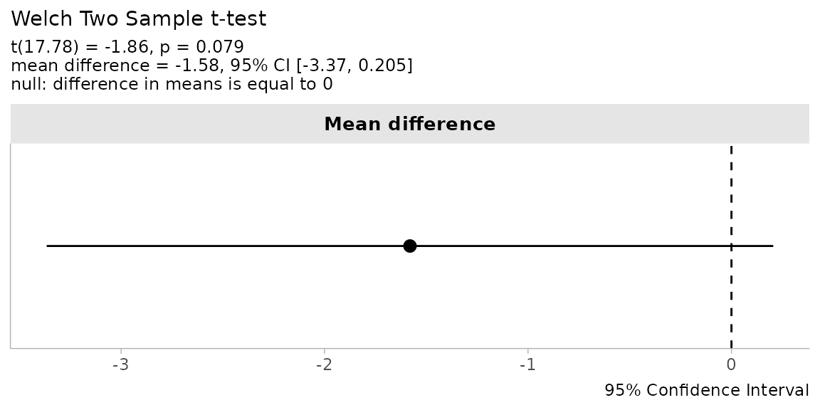

For equivalence tests, the plot displays both equivalence bounds as dashed reference lines:

plot_htest_est(res_equiv)

Set describe = FALSE for a cleaner plot without the statistical summary in the subtitle:

plot_htest_est(res_equiv, describe = FALSE)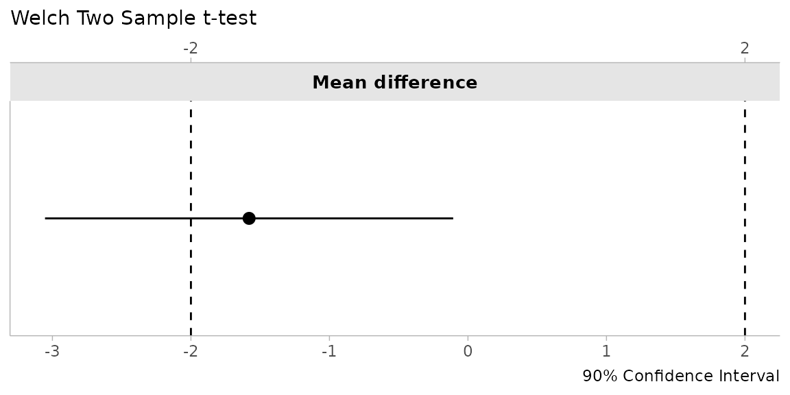

Because the result is a ggplot2 object, you can customize it further with standard ggplot2 functions.

Putting It All Together

Here is a compact workflow tying together the full set of tools. We run an equivalence test, tabulate the result, describe it in text, and visualize it:

# Run equivalence test
result <- simple_htest(extra ~ group,
                       data = sleep,
                       mu = 2,
                       alternative = "equivalence")

# Tabulate
df_htest(result)
#>                    method         t       df   p.value mean difference       SE
#> 1 Welch Two Sample t-test 0.4946466 17.77647 0.3134536           -1.58 0.849091
#>    lower.ci   upper.ci conf.level alternative null1 null2
#> 1 -3.053381 -0.1066185        0.9 equivalence    -2     2

# Describe
describe_htest(result)
#> [1] "The Welch Two Sample t-test is not statistically significant (t(17.776) = 0.495, p = 0.313, mean of group '1' = 0.75, mean of group '2' = 2.33, mean difference ('1' - '2') = -1.58, 90% C.I.[-3.05, -0.107]) at a 0.05 alpha-level. The null hypothesis cannot be rejected. At the desired error rate, it cannot be stated that the true difference in means is between -2 and 2."

# Visualize
plot_htest_est(result)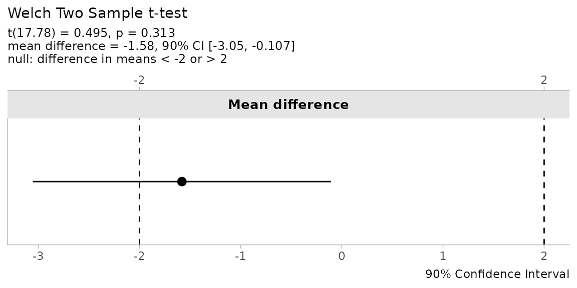

TOSTER provides a consistent, informative interface for hypothesis testing that goes well beyond equivalence. Whether you need a standard t-test with better output, a non-inferiority analysis, or a full TOST procedure, the same tools apply.