Robust TOST Procedures

Introduction to Robust TOST Methods

The Two One-Sided Tests (TOST) procedure is a statistical approach used to test for equivalence between groups or conditions. Unlike traditional null hypothesis significance testing (NHST) which aims to detect differences, TOST is designed to statistically demonstrate similarity or equivalence within predefined bounds.

While the standard t_TOST function in TOSTER provides a parametric approach to equivalence testing, it relies on assumptions of normality and homogeneity of variance. In real-world data analysis, these assumptions are often violated, necessitating more robust alternatives. This vignette introduces several robust TOST methods available in the TOSTER package that maintain their validity under a wider range of data conditions.

Choosing by Estimand

Before selecting a robust method, it is worth clarifying what quantity your equivalence bounds are intended to constrain. Different methods target different estimands, and the bounds only have their intended meaning when matched to the right one. If your bounds refer to mean differences, a permutation t-test or bootstrap approach is appropriate. If they refer to trimmed mean differences due to concerns about heavy tails (outliers), Yuen’s trimmed bootstrap or permutation test are natural choices. If you are interested in stochastic dominance (P(X > Y)), the Brunner-Munzel test provides a transparent framework. The Wilcoxon-Mann-Whitney and Hodges-Lehmann procedures target the pseudo-median of pairwise differences, which coincides with mean and median differences only under a location shift assumption. When that assumption is violated, bounds set on the pseudo-median may not correspond to the magnitude of difference in means or medians that you intended to declare equivalent.

TL;DR choose your test carefully and this should be informed by the estimand of interest.

When to Use Robust TOST Methods

Consider using the robust alternatives to t_TOST when:

Your data shows notable departures from normality (e.g., skewed distributions, heavy tails)
Potential outliers are a concern
Sample sizes are small or unequal
You have concerns about violating the assumptions of parametric tests
You want to confirm parametric test results with complementary nonparametric approaches

The following table provides a quick overview of the robust methods covered in this vignette:

Method	Function	Key Characteristics	Best Used When
Wilcoxon TOST	`wilcox_TOST()`	Rank-based, nonparametric	Ordinal data; see caveats below
Brunner-Munzel	`brunner_munzel()`	Probability-based, robust to heteroscedasticity	Stochastic superiority is the effect of interest
Hodges-Lehmann	`hodges_lehmann()`	Robust location estimator, permutation or asymptotic	Robust location shift testing, outlier resistance
Permutation t-test	`perm_t_test()`	Resampling without replacement, exact p-values possible	Small samples, mean differences, exact inference
Bootstrap TOST	`boot_t_TOST()`	Resampling with replacement, flexible	Moderate samples, mean differences, visualization
Log-Transformed TOST	`log_TOST()`	Ratio-based, for multiplicative comparisons	Comparing relative differences (e.g., bioequivalence)
SES estimation/testing	`ses_calc()` / `boot_ses_calc()`	Non-parametric effect sizes with optional hypothesis testing	Testing on the effect size scale directly

Wilcoxon-Mann-Whitney TOST

The Wilcoxon group of tests (includes Mann-Whitney U-test) provide a non-parametric test of differences between groups, or within samples, based on ranks. With TOST, there are two separate tests of directional location shift to determine if the location shift is within (equivalence) or outside (minimal effect). The exact calculations can be explored via the documentation of the wilcox.test function.

Why WMW Tests Can Be Misleading

While the Wilcoxon-Mann-Whitney (WMW) tests are widely used as the “non-parametric alternative” to the t-test, there are important reasons to be cautious about their interpretation, particularly in the equivalence testing context.

What WMW actually tests

A common misconception is that the WMW test compares medians (see Karch 2021; Divine et al. 2018). Without additional assumptions, the two-tailed WMW test is a test of stochastic equality:

\[ H_0: p = \Pr(X < Y) + \frac{1}{2}\Pr(X = Y) = 0.5 \]

where \(X\) and \(Y\) are randomly selected observations from the two groups. This quantity \(\hat{p} = U / (n_1 \cdot n_2)\) (where \(U\) is the Mann-Whitney U statistic) has nothing directly to do with means, medians, or even the shapes of the distributions. It is the only interpretation that holds without additional assumptions.

Only under a location-shift assumption (the two distributions have identical shapes, differing only in location) does the WMW test become a test about the Hodges-Lehmann pseudomedian of pairwise differences. And only if the distributions are additionally symmetric can this be interpreted as a test of median or mean differences.

Counterexamples

Divine et al. (2018) demonstrate several scenarios that illustrate the disconnect between the WMW test and medians:

Equal medians, significant WMW test: Both groups can have the same median yet the WMW test rejects \(H_0\) (\(p < 0.001\)), because the distributions differ in shape.
Very different medians, non-significant WMW test: Samples can have medians of 9 vs. 99, yet \(\hat{p} \approx 0.5\) with \(p \approx 1.0\), because neither group stochastically dominates the other.
Significance in the wrong direction: The group with the higher median can have \(\hat{p} > 0.5\), meaning the WMW test suggests the opposite direction from the median comparison.

The problem for equivalence testing

This interpretive difficulty is especially pronounced for equivalence testing. When we perform TOST with Wilcoxon tests via wilcox_TOST, the equivalence bounds are applied to the pseudo-median of pairwise differences. But this quantity corresponds to the difference in means or medians only under the location shift assumption. When distributions differ in shape, a bound of \(\pm 2\) units on the pseudo-median of pairwise differences does not guarantee that means or medians are within \(\pm 2\) of each other. The researcher may believe they are bounding mean or median differences when they are in fact bounding a different quantity entirely.

What to use instead

For differences in means (or trimmed means): Use perm_t_test or boot_t_TOST. These test hypotheses directly about means while relaxing some distributional assumptions.

For stochastic superiority: Use brunner_munzel, which provides a clearer framework with an interpretable effect size (the relative effect, \(\hat{p}\)) and directly supports equivalence and minimal effect testing.

For robust location testing: Use hodges_lehmann, which explicitly tests the Hodges-Lehmann estimator with permutation or asymptotic inference and makes the location-shift assumption transparent.

For testing effect sizes directly: Use ses_calc to estimate and test non-parametric standardized effect sizes (rank-biserial correlation, WMW odds, concordance) with proper hypothesis testing support.

The wilcox_TOST function remains available for situations where rank-based tests are specifically desired, such as with ordinal data or when consistency with prior analyses that used WMW tests is needed.

Key Features and Usage

TOSTER’s version is the wilcox_TOST function. Overall, this function operates extremely similar to the t_TOST function. However, the standardized mean difference (SMD) is not calculated. Instead the rank-biserial correlation is calculated for all types of comparisons (e.g., two sample, one sample, and paired samples). Also, there is no plotting capability at this time for the output of this function.

Understanding the Equivalence Bounds (`eqb`)

The equivalence bounds (eqb) are specified on the raw scale of your data, just like the mu argument in stats::wilcox.test(). This means eqb represents actual differences in location (e.g., location shifts) in the original units of measurement, not standardized effect sizes. Unlike t_TOST, where eqb can be set in terms of standardized mean differences (e.g., Cohen’s d), in wilcox_TOST, you must define eqb based on the scale of your data for wilcox_TOST.

The eqb and ses parameters are completely independent:

eqb sets the equivalence bounds on the raw data scale for the statistical test
ses only determines which type of standardized effect size is calculated and reported (e.g., rank-biserial correlation, concordance probability, or odds)
Changing ses does not change the meaning or interpretation of eqb

As an example, we can use the sleep data to make a non-parametric comparison of equivalence.

data('sleep')
library(TOSTER)

test1 = wilcox_TOST(formula = extra ~ group,
                      data = sleep,
                      eqb = .5)


print(test1)

## 
## Wilcoxon rank sum test with continuity correction
## 
## The equivalence test was non-significant W = 20.000, p = 8.94e-01
## The null hypothesis test was non-significant W = 25.500, p = 6.93e-02
## NHST: don't reject null significance hypothesis that the effect is equal to zero 
## TOST: don't reject null equivalence hypothesis
## 
## TOST Results 
##            Test Statistic p.value
## NHST                 25.5   0.069
## TOST Lower           34.0   0.894
## TOST Upper           20.0   0.013
## 
## Effect Sizes 
##                           Estimate              C.I. Conf. Level
## Median of Differences       -1.346      [-3.4, -0.1]         0.9
## Rank-Biserial Correlation   -0.490 [-0.757, -0.0561]         0.9

Interpreting the Results

When interpreting the output of wilcox_TOST, pay attention to:

The p-values for both one-sided tests (p1 and p2)
The equivalence test p-value (TOSTp), which should be < alpha to claim equivalence
The rank-biserial correlation (rb) and its confidence interval

A statistically significant equivalence test (p < alpha) indicates that the observed effect is statistically within your specified equivalence bounds. The rank-biserial correlation provides a measure of effect size, with values ranging from -1 to 1 much like any correlation coefficient. A value of 0 indicates no difference between groups, while values closer to -1 or 1 indicate stronger effects in either direction. The confidence interval for the rank-biserial correlation can help you understand the precision of your standarized effect size estimate.

Standardized Effect Sizes

The wilcox_TOST function reports a standardized effect size (SES) alongside the equivalence test. By default, this is the rank-biserial correlation, but you can select other effect sizes (concordance probability, WMW odds, or WMW log-odds) via the ses argument. Changing ses only affects which effect size is reported; it does not change the equivalence test itself.

# Rank biserial
wilcox_TOST(formula = extra ~ group,
                      data = sleep,
                      ses = "r",
                      eqb = .5)

## 
## Wilcoxon rank sum test with continuity correction
## 
## The equivalence test was non-significant W = 20.000, p = 8.94e-01
## The null hypothesis test was non-significant W = 25.500, p = 6.93e-02
## NHST: don't reject null significance hypothesis that the effect is equal to zero 
## TOST: don't reject null equivalence hypothesis
## 
## TOST Results 
##            Test Statistic p.value
## NHST                 25.5   0.069
## TOST Lower           34.0   0.894
## TOST Upper           20.0   0.013
## 
## Effect Sizes 
##                           Estimate              C.I. Conf. Level
## Median of Differences       -1.346      [-3.4, -0.1]         0.9
## Rank-Biserial Correlation   -0.490 [-0.757, -0.0561]         0.9

# Odds
wilcox_TOST(formula = extra ~ group,
                      data = sleep,
                      ses = "o",
                      eqb = .5)

## 
## Wilcoxon rank sum test with continuity correction
## 
## The equivalence test was non-significant W = 20.000, p = 8.94e-01
## The null hypothesis test was non-significant W = 25.500, p = 6.93e-02
## NHST: don't reject null significance hypothesis that the effect is equal to zero 
## TOST: don't reject null equivalence hypothesis
## 
## TOST Results 
##            Test Statistic p.value
## NHST                 25.5   0.069
## TOST Lower           34.0   0.894
## TOST Upper           20.0   0.013
## 
## Effect Sizes 
##                       Estimate             C.I. Conf. Level
## Median of Differences  -1.3464     [-3.4, -0.1]         0.9
## WMW Odds                0.3423 [0.1383, 0.8937]         0.9

# Concordance
wilcox_TOST(formula = extra ~ group,
                      data = sleep,
                      ses = "c",
                      eqb = .5)

## 
## Wilcoxon rank sum test with continuity correction
## 
## The equivalence test was non-significant W = 20.000, p = 8.94e-01
## The null hypothesis test was non-significant W = 25.500, p = 6.93e-02
## NHST: don't reject null significance hypothesis that the effect is equal to zero 
## TOST: don't reject null equivalence hypothesis
## 
## TOST Results 
##            Test Statistic p.value
## NHST                 25.5   0.069
## TOST Lower           34.0   0.894
## TOST Upper           20.0   0.013
## 
## Effect Sizes 
##                       Estimate             C.I. Conf. Level
## Median of Differences   -1.346     [-3.4, -0.1]         0.9
## Concordance              0.255 [0.1215, 0.4719]         0.9

For details on how each effect size is calculated, the available confidence interval methods, and how to perform hypothesis testing directly on the effect size scale, see the [Standardized Effect Sizes: Estimation and Testing] section later in this vignette.

Interface with `wilcox.test`

You can also just directly use wilcox.test through the simple_htest function. This might be useful if you find the interface of wilcox.test more intuitive for certain applications than wilcox_TOST, or if you want to perform a standard WMW test without the TOST framework.

simple_htest(formula = extra ~ group,
                      data = sleep,
                      test = "w", alternative = "e",
                      mu = .5)

## Warning in wilcox.test.default(x = x, y = y, paired = paired, mu = 0, conf.int
## = TRUE, : cannot compute exact p-value with ties

## Warning in wilcox.test.default(x = x, y = y, paired = paired, mu = 0, conf.int
## = TRUE, : cannot compute exact confidence intervals with ties

## 
##  Wilcoxon rank sum exact test
## 
## data:  extra by group
## W = 34, p-value = 0.8912
## alternative hypothesis: equivalence
## null values:
## location shift location shift 
##           -0.5            0.5 
## 90 percent confidence interval:
##  -3.39996507 -0.09995341
## sample estimates:
## Hodges-Lehmann estimate ('1' - '2') 
##                           -1.346388

Brunner-Munzel Test

As Karch (2021) explained, there are some reasons to dislike the Wilcoxon-Mann-Whitney (WMW) family of tests as the non-parametric alternative to the t-test. Regardless of the underlying statistical arguments¹, it can be argued that the interpretation of the WMW tests, especially when involving equivalence testing, is difficult. Some may want a non-parametric alternative to the WMW test, and the Brunner-Munzel test(s) may be a useful option.

Overview and Advantages

The Brunner-Munzel test (Brunner and Munzel 2000; Neubert and Brunner 2007) offers several advantages over the Wilcoxon-Mann-Whitney tests:

It does not assume equal distributions (shapes) between groups
It is robust to heteroscedasticity (unequal variances)
It provides a more interpretable effect size measure (the “relative effect”)
It maintains good statistical properties even with unequal sample sizes

The Brunner-Munzel test is based on calculating the “stochastic superiority” (Karch 2021), which is usually referred to as the relative effect, based on the ranks of the two groups being compared (X and Y). A Brunner-Munzel type test is then a directional test of an effect, and answers a question akin to “what is the probability that a randomly sampled value of X will be greater than Y?”²

\[ \hat p = P(X>Y) + 0.5 \cdot P(X=Y) \]

Where:

\(P(X>Y)\) is the probability that a random value from X exceeds a random value from Y
\(P(X=Y)\) is the probability that random values from X and Y are equal
The 0.5 factor means ties contribute half their weight to the probability

The relative effect \(\hat p\) has an intuitive interpretation:

\(\hat p = 0.5\) indicates no difference between groups (stochastic equality)
\(\hat p > 0.5\) indicates values in X tend to be greater than values in Y
\(\hat p < 0.5\) indicates values in X tend to be smaller than values in Y

Basics of the Calculative Approach

A studentized test statistic can be calculated as:

\[ t = \sqrt{N} \cdot \frac{\hat p - p_{null}}{s} \]

Where:

\(N\) is the total sample size
\(\hat p\) is the estimated relative effect
\(p_{null}\) is the null hypothesis value (typically 0.5)
\(s\) is the rank-based Brunner-Munzel standard error

The default null hypothesis \(p_{null}\) is typically 0.5 (50% probability of superiority (tie) is the default null), and \(s\) refers to the rank-based Brunner-Munzel standard error. The null can be modified, thereby allowing for equivalence testing directly based on the relative effect. Additionally, for paired samples the probability of superiority is based on a hypothesis of exchangeability and is not based on the difference scores³.

For more details on the calculative approach, I suggest reading Karch (2021). At small sample sizes, it is recommended that the permutation version of the test (test_method = "perm") be used rather than the basic test statistic approach.

Test Methods

The brunner_munzel function provides three test methods via the test_method argument:

“t” (default): Uses a t-distribution approximation with Satterthwaite-Welch degrees of freedom. This is appropriate for moderate to large sample sizes (generally n ≥ 15 per group).
“logit”: Uses a logit transformation to produce range-preserving confidence intervals that are guaranteed to stay within [0, 1]. This method is recommended when the estimated relative effect is close to 0 or 1.
“perm”: A studentized permutation test following Neubert and Brunner (2007). This method is highly recommended when sample sizes are small (< 15 per group) as it provides better control of Type I error rates in these situations.

Examples

Basic Two-Sample Test

The interface for the function is similar to t.test. The brunner_munzel function allows for standard hypothesis tests (“two.sided”, “less”, “greater”) as well as equivalence and minimal effect tests.

# Default studentized test (t-approximation)
brunner_munzel(formula = extra ~ group,
               data = sleep)

## Sample size in at least one group is small. Permutation test (test_method = 'perm') is highly recommended.

## 
##  Two-sample Brunner-Munzel test
## 
## data:  extra by group
## t = -2.1447, df = 16.898, p-value = 0.04682
## alternative hypothesis: true relative effect is not equal to 0.5
## 95 percent confidence interval:
##  0.01387048 0.49612952
## sample estimates:
## P('1'>'2') + .5*P('1'='2') 
##                      0.255

# Permutation test (recommended for small samples)
brunner_munzel(formula = extra ~ group,
               data = sleep,
               test_method = "perm")

## 
##  Two-sample Brunner-Munzel Randomization test
## 
## data:  extra by group
## t-observed = -2.1447, N-permutations = 10000, p-value = 0.05739
## alternative hypothesis: true relative effect is not equal to 0.5
## 95 percent confidence interval:
##  0.002772424 0.509273251
## sample estimates:
## P('1'>'2') + .5*P('1'='2') 
##                      0.255

Logit Transformation for Range-Preserving CIs

When the relative effect estimate is close to 0 or 1, the standard confidence intervals may extend beyond the valid [0, 1] range. The logit transformation method addresses this:

# Logit transformation for range-preserving CIs
brunner_munzel(formula = extra ~ group,
               data = sleep,
               test_method = "logit")

## Sample size in at least one group is small. Permutation test (test_method = 'perm') is highly recommended.

## 
##  Two-sample Brunner-Munzel test (logit)
## 
## data:  extra by group
## t = -1.7829, df = 16.898, p-value = 0.09257
## alternative hypothesis: true relative effect is not equal to 0.5
## 95 percent confidence interval:
##  0.08775255 0.54912824
## sample estimates:
## P('1'>'2') + .5*P('1'='2') 
##                      0.255

Equivalence Testing

The brunner_munzel function directly supports equivalence testing via the alternative argument. For equivalence tests, you specify bounds for the relative effect using the mu argument:

# Equivalence test: is the relative effect between 0.3 and 0.7?
brunner_munzel(formula = extra ~ group,
               data = sleep,
               alternative = "equivalence",
               mu = c(0.3, 0.7))

## Sample size in at least one group is small. Permutation test (test_method = 'perm') is highly recommended.

## 
##  Two-sample Brunner-Munzel test
## 
## data:  extra by group
## t = -0.39392, df = 16.898, p-value = 0.6507
## alternative hypothesis: equivalence
## null values:
## lower bound upper bound 
##         0.3         0.7 
## 90 percent confidence interval:
##  0.0562039 0.4537961
## sample estimates:
## P('1'>'2') + .5*P('1'='2') 
##                      0.255

# Permutation-based equivalence test
brunner_munzel(formula = extra ~ group,
               data = sleep,
               alternative = "equivalence",
               mu = c(0.3, 0.7),
               test_method = "perm")

## NOTE: Permutation-based TOST for equivalence/minimal.effect testing.

## 
##  Two-sample Brunner-Munzel Randomization test
## 
## data:  extra by group
## t-observed = -0.39392, N-permutations = 10000, p-value = 0.6528
## alternative hypothesis: equivalence
## null values:
## lower bound upper bound 
##         0.3         0.7 
## 90 percent confidence interval:
##  0.05980676 0.45019324
## sample estimates:
## P('1'>'2') + .5*P('1'='2') 
##                      0.255

Minimal Effect Testing

You can also test whether the relative effect falls outside specified bounds (minimal effect test):

# Minimal effect test: is the relative effect outside 0.4 to 0.6?
brunner_munzel(formula = extra ~ group,
               data = sleep,
               alternative = "minimal.effect",
               mu = c(0.4, 0.6))

## Sample size in at least one group is small. Permutation test (test_method = 'perm') is highly recommended.

## 
##  Two-sample Brunner-Munzel test
## 
## data:  extra by group
## t = -1.2693, df = 16.898, p-value = 0.1108
## alternative hypothesis: minimal.effect
## null values:
## lower bound upper bound 
##         0.4         0.6 
## 90 percent confidence interval:
##  0.0562039 0.4537961
## sample estimates:
## P('1'>'2') + .5*P('1'='2') 
##                      0.255

Paired Samples

The Brunner-Munzel test can also be applied to paired samples using the paired argument. Note that for paired samples, the test is based on a hypothesis of exchangeability:

# Paired samples test
brunner_munzel(x = sleep$extra[sleep$group == 1],
               y = sleep$extra[sleep$group == 2],
               paired = TRUE)

## Sample size in at least one group is small. Permutation test (test_method = 'perm') is highly recommended.

## 
##  Paired Brunner-Munzel test
## 
## data:  sleep$extra[sleep$group == 1] and sleep$extra[sleep$group == 2]
## t = -3.7266, df = 9, p-value = 0.004722
## alternative hypothesis: true relative effect is not equal to 0.5
## 95 percent confidence interval:
##  0.1062776 0.4037224
## sample estimates:
## P(X>Y) + .5*P(X=Y) 
##              0.255

# Paired samples with permutation test
brunner_munzel(x = sleep$extra[sleep$group == 1],
               y = sleep$extra[sleep$group == 2],
               paired = TRUE,
               test_method = "perm")

## 
##  Paired Brunner-Munzel Exact Permutation test
## 
## data:  sleep$extra[sleep$group == 1] and sleep$extra[sleep$group == 2]
## t-observed = -3.7266, N-permutations = 1024, p-value = 0.003906
## alternative hypothesis: true relative effect is not equal to 0.5
## 95 percent confidence interval:
##  0.1233862 0.3866138
## sample estimates:
## P(X>Y) + .5*P(X=Y) 
##              0.255

Testing Against a Non-Standard Null

You can test against null values other than 0.5:

# Test if the relative effect differs from 0.3
brunner_munzel(formula = extra ~ group,
               data = sleep,
               mu = 0.3)

## Sample size in at least one group is small. Permutation test (test_method = 'perm') is highly recommended.

## 
##  Two-sample Brunner-Munzel test
## 
## data:  extra by group
## t = -0.39392, df = 16.898, p-value = 0.6986
## alternative hypothesis: true relative effect is not equal to 0.3
## 95 percent confidence interval:
##  0.01387048 0.49612952
## sample estimates:
## P('1'>'2') + .5*P('1'='2') 
##                      0.255

Interpreting Brunner-Munzel Results

When interpreting the Brunner-Munzel test results:

The relative effect (p-hat) is the primary measure of interest
Values near 0.5 suggest no tendency for one group to produce larger values than the other
For equivalence testing, you are testing whether this relative effect falls within your specified bounds
A significant equivalence test suggests that the probability of superiority is statistically confined to your specified range

Choosing the Right Test Method

Use test_method = "t" when:

Sample sizes are moderate to large (n ≥ 15 per group)
You want the fastest computation
The relative effect estimate is not near the boundaries [0, 1]

Use test_method = "logit" when:

The relative effect estimate is close to 0 or 1
You need confidence intervals guaranteed to stay within [0, 1]
Sample sizes are moderate to large

Use test_method = "perm" when:

Sample sizes are small (n < 15 per group)
You want better Type I error control in small samples
Precision is more important than computational speed

Note that the permutation approach can be computationally intensive for large datasets. Additionally, with a permutation test you may observe situations where the confidence interval and the p-value would yield different conclusions though they should closely match in most cases.

Non-Inferiority Testing

The Brunner-Munzel test can be used for non-inferiority testing with ordered categorical data (Munzel and Hauschke 2003). By setting appropriate bounds, you can test whether a new treatment is not relevantly inferior to a standard:

# Example: test non-inferiority with lower bound of 0.35
# (i.e., the new treatment should not be substantially worse)
brunner_munzel(formula = extra ~ group,
               data = sleep,
               alternative = "greater",
               mu = 0.35)

## Sample size in at least one group is small. Permutation test (test_method = 'perm') is highly recommended.

## 
##  Two-sample Brunner-Munzel test
## 
## data:  extra by group
## t = -0.83161, df = 16.898, p-value = 0.7914
## alternative hypothesis: true relative effect is greater than 0.35
## 95 percent confidence interval:
##  0.0562039 1.0000000
## sample estimates:
## P('1'>'2') + .5*P('1'='2') 
##                      0.255

Hodges-Lehmann Estimator and Test

The hodges_lehmann function provides a robust location test based on the Hodges-Lehmann estimator (Hodges and Lehmann 1963; Fried and Dehling 2011). This is a natural companion to the WMW discussion above: while wilcox_TOST implicitly relies on the location-shift assumption without making it explicit, hodges_lehmann directly estimates and tests the location shift parameter with transparent assumptions.

Why Use the Hodges-Lehmann Estimator?

The Hodges-Lehmann estimator has several appealing properties:

Robustness to outliers The Hodges-Lehmann estimator has bounded influence, meaning individual extreme observations cannot arbitrarily distort the estimate. This provides substantially greater robustness than the mean while retaining higher efficiency than the median under normal distributions.
Efficiency: Under normality, the Hodges-Lehmann estimator achieves about 95.5% of the efficiency of the sample mean, a small price for substantial robustness gains.
Transparent assumptions and distinct inference: Unlike wilcox_TOST, which uses the standard Wilcoxon rank-sum test (and whose confidence interval is obtained by inverting that same test), hodges_lehmann constructs its test statistic by dividing the HL estimator by a robust scale estimate following Fried and Dehling (2011). This means that hodges_lehmann and wilcox_TOST can yield different inferential conclusions despite sharing the same point estimator, particularly in the presence of outliers or heteroscedasticity. The Fried-Dehling approach trades the exact test-CI duality of the WMW framework for greater robustness to contamination.

Estimators

For one-sample and paired designs, the function computes the HL1 estimator, the median of all Walsh averages (pairwise averages including self-pairs):

\[ \hat{\theta}_{HL1} = \text{med}\left\{\frac{X_i + X_j}{2} : 1 \leq i \leq j \leq n\right\} \]

For two-sample designs, the function computes the HL2 estimator, the median of all pairwise differences between samples:

\[ \hat{\Delta}_{HL2} = \text{med}\{Y_j - X_i : i = 1, \ldots, m; \; j = 1, \ldots, n\} \]

Both estimators are consistent with the pseudomedian and location shift estimates returned by wilcox.test.

Interpreting the Estimand

It is important to understand what these estimators target, particularly for equivalence testing where the meaning of your bounds depends on the estimand.

Two-sample (HL2): The HL2 estimates the median of the distribution of \(X - Y\), where \(X\) and \(Y\) are independently drawn from their respective populations. In practical terms, if you repeatedly drew one observation from each group and computed the difference, the HL2 gives the value around which half of those pairwise differences would fall above and half below. This is not the same as the difference in population medians (\(\text{median}(X) - \text{median}(Y)\)), nor the difference in means. These quantities coincide under a location shift model but diverge when distributional shapes differ.

One-sample and paired (HL1): The HL1 estimates the pseudo-median of the distribution, defined as the median of \((D + D') / 2\) where \(D\) and \(D'\) are independent draws from the same distribution. This is a measure of the center of symmetry rather than the 50th percentile. Under symmetry, the pseudo-median, median, and mean coincide. Under skewness, they do not. For paired equivalence testing, the question being answered is whether the pseudo-median of the within-subject difference distribution falls within the equivalence bounds, which is a subtly different question than whether the median or mean change score is small.

Implications for equivalence bounds: When setting equivalence bounds for hodges_lehmann, you are bounding the pseudo-median of pairwise differences (two-sample) or the pseudo-median of within-subject differences (paired). Under the location shift assumption, these correspond directly to the difference in means or medians, and bounds have their intuitive interpretation. Without this assumption, a bound of \(\pm 2\) on the pseudo-median does not guarantee that means or medians are within \(\pm 2\) of each other. If your equivalence question is specifically about means, consider perm_t_test or boot_t_TOST instead. If it is about stochastic dominance, consider brunner_munzel.

Test Methods

The hodges_lehmann function supports three inference approaches controlled by the R argument:

Asymptotic test (R = NULL, the default): Uses kernel density estimation to approximate the variance of the Hodges-Lehmann estimator. Suitable for moderate to large samples (n \(\geq\) 30 per group). Note that this produces confidence intervals that will differ from wilcox.test due to the different variance estimation method.
Exact permutation test (R \(\geq\) max permutations): Enumerates all possible permutations and provides exact p-values using an unstudentized approach.
Randomization test (R < max permutations): Samples R permutations with replacement. Uses the (b+1)/(R+1) formula by default for exact Type I error control (Phipson and Smyth 2010) and is also a unstudentized approach.

Examples

Basic Two-Sample Test

data('sleep')

# Asymptotic Hodges-Lehmann test
hodges_lehmann(formula = extra ~ group,
               data = sleep)

## 
##  Asymptotic Hodges-Lehmann Two Sample Test
## 
## data:  extra by group
## Z = -1.3179, p-value = 0.1875
## alternative hypothesis: true location is not equal to 0
## 95 percent confidence interval:
##  -3.3576425  0.6576425
## sample estimates:
## Hodges-Lehmann estimate ('1' - '2') 
##                               -1.35

Permutation-Based Test

For small samples, the permutation approach is recommended:

# Permutation test
hodges_lehmann(formula = extra ~ group,
               data = sleep,
               R = 1999)

## 
##  Randomization Hodges-Lehmann Two Sample Test
## 
## data:  extra by group
## Z = -0.72973, p-value = 0.1275
## alternative hypothesis: true location is not equal to 0
## 95 percent confidence interval:
##  -3.15  0.50
## sample estimates:
## Hodges-Lehmann estimate ('1' - '2') 
##                               -1.35

Equivalence Testing

The function directly supports equivalence testing via the alternative argument. Equivalence bounds are specified on the pseudomedian (or location shift) scale:

# Equivalence test: is the location shift within ±2 units?
# Equivalence/minimal.effect alternatives use the asymptotic method only
hodges_lehmann(formula = extra ~ group,
               data = sleep,
               alternative = "equivalence",
               mu = 2)

## 
##  Asymptotic Hodges-Lehmann Two Sample Test
## 
## data:  extra by group
## Z = 0.63456, p-value = 0.2629
## alternative hypothesis: equivalence
## null values:
## location location 
##       -2        2 
## 90 percent confidence interval:
##  -3.0348667  0.3348667
## sample estimates:
## Hodges-Lehmann estimate ('1' - '2') 
##                               -1.35

Note on equivalence testing: Equivalence and minimal effect tests are only available with the asymptotic method (R = NULL). Permutation tests are not supported for these alternatives because the scale estimators (S1, S2) from Fried and Dehling (2011) do not produce a pivotal test statistic for the Hodges-Lehmann estimator. Without pivotality, the permutation distribution generated under the exchangeability null is not a valid reference distribution for testing at the equivalence bounds. This limitation compounds with the inherent conservatism of the naive intersection-union procedure, potentially yielding substantial power loss. The asymptotic method uses kernel density estimation to approximate the standard error, which provides a proper pivot and valid boundary-null inference.

Paired Samples

# Paired Hodges-Lehmann test
hodges_lehmann(x = sleep$extra[sleep$group == 1],
               y = sleep$extra[sleep$group == 2],
               paired = TRUE,
               R = 1999)

## Computing all 1024 exact permutations.

## 
##  Exact Permutation Hodges-Lehmann Paired Test
## 
## data:  sleep$extra[sleep$group == 1] and sleep$extra[sleep$group == 2]
## Z = -1.3, p-value < 2.2e-16
## alternative hypothesis: true location is not equal to 0
## 95 percent confidence interval:
##  -1.8 -0.8
## sample estimates:
## Hodges-Lehmann estimate (z = x - y) 
##                                -1.3

Minimal Effect Testing

# Minimal effect test: is the location shift outside ±0.5?
# Minimal effect alternative uses the asymptotic method only
hodges_lehmann(formula = extra ~ group,
               data = sleep,
               alternative = "minimal.effect",
               mu = 0.5)

## 
##  Asymptotic Hodges-Lehmann Two Sample Test
## 
## data:  extra by group
## Z = -0.82981, p-value = 0.2033
## alternative hypothesis: minimal.effect
## null values:
## location location 
##     -0.5      0.5 
## 90 percent confidence interval:
##  -3.0348667  0.3348667
## sample estimates:
## Hodges-Lehmann estimate ('1' - '2') 
##                               -1.35

Choosing the Right Approach

Use the asymptotic test (R = NULL) when:

Sample sizes are moderate to large (n \(\geq\) 30 per group)
You want the fastest computation
Distributions are not extremely heavy-tailed or skewed
When the null != 0 or when the alternative is “equivalence” or “minimal.effect”

Use the permutation test (R \(\geq\) max permutations) when:

Sample sizes are small enough for exact enumeration
You want exact p-values with no Monte Carlo error
For one-sample/paired: \(n \leq 16\) (\(2^{16}\) = 65,536 permutations)

Use the randomization test (set R to a large number) when:

Exact permutation is too computationally expensive
You want distribution-free inference without asymptotic assumptions

Resampling Methods: Bootstrapping and Permutation

Resampling methods provide robust alternatives to parametric t-tests by using the data itself to approximate the sampling distribution of the test statistic. TOSTER offers two complementary resampling approaches: bootstrapping and permutation testing. While both methods relax distributional assumptions, they differ in their mechanics and are suited to different situations.

Conceptual Overview

Bootstrapping resamples with replacement from the observed data to estimate the variability of a statistic. The bootstrap distribution approximates what we would see if we could repeatedly sample from the true population. This approach is particularly useful when you want confidence intervals and effect size estimates alongside your p-values.

Permutation testing resamples without replacement by randomly reassigning observations to groups (or flipping signs for one-sample/paired tests). Under the null hypothesis of no difference, group labels are exchangeable, and the permutation distribution represents the exact null distribution. Permutation tests provide valid inference even with very small samples where asymptotic approximations may fail.

When to Use Each Method

Scenario	Recommended Method	Rationale
Very small samples (paired/one-sample N < 17, two-sample N < 20)	Permutation	Exact permutations are computationally feasible and provide exact p-values
Moderate to large samples	Bootstrap	More computationally efficient; provides stable CI estimates
Outliers present	Permutation with trimming	Combines exact inference with robust location estimation
Complex data structures	Bootstrap	More flexible for non-standard designs
Publication requiring exact p-values	Permutation (if feasible)	No Monte Carlo error when exact permutations computed

The sample size thresholds above reflect computational practicality. For one-sample or paired tests, the number of possible sign permutations is \(2^n\), which equals 65,536 when n = 16 and jumps to 131,072 at n = 17. For two-sample tests, the number of possible group assignments is \(\binom{n_x + n_y}{n_x}\), which grows even faster. When exact enumeration is feasible, permutation tests yield exact p-values with no Monte Carlo error.

Permutation t-test

The perm_t_test function implements studentized permutation tests following the approaches of Janssen (1997) and Chung and Romano (2013). The studentized approach computes a t-statistic for each permutation, making the test valid even under heteroscedasticity (unequal variances).

Permutation Procedure

For one-sample and paired tests, permutation is performed by randomly flipping the signs of the centered observations (or difference scores). Under the null hypothesis that the mean equals the hypothesized value, positive and negative deviations are equally likely, making sign assignments exchangeable.

For two-sample tests, permutation is performed by randomly reassigning observations to the two groups. Under the null hypothesis of no group difference, group membership is arbitrary, making the labels exchangeable.

Two-Sample Permutation Algorithm

The studentized permutation test for two independent samples proceeds as follows:

Compute the observed test statistic from the original data. For the standard case (no trimming, unequal variances allowed):

\[ t_{obs} = \frac{\bar{x} - \bar{y} - \mu_0}{\sqrt{s_x^2/n_x + s_y^2/n_y}} \]

Where \(\bar{x}\) and \(\bar{y}\) are the sample means, \(s_x^2\) and \(s_y^2\) are the sample variances, \(n_x\) and \(n_y\) are the sample sizes, and \(\mu_0\) is the null hypothesis value (typically 0).

Pool the observations: \(z = (x_1, \ldots, x_{n_x}, y_1, \ldots, y_{n_y})\)
For each permutation \(b = 1, \ldots, B\):
- Randomly assign \(n_x\) observations to group X and the remaining \(n_y\) to group Y
- Compute the permutation means \(\bar{x}^{*b}\) and \(\bar{y}^{*b}\)
- Compute the permutation variances \(s_x^{*2b}\) and \(s_y^{*2b}\)
- Compute the permutation test statistic:

\[ t^{*b} = \frac{\bar{x}^{*b} - \bar{y}^{*b}}{\sqrt{s_x^{*2b}/n_x + s_y^{*2b}/n_y}} \]

Compute the p-value as the proportion of permutation statistics as extreme as or more extreme than the observed statistic.

Welch Variant (var.equal = FALSE)

When var.equal = FALSE (the default), the standard error is computed separately for each group as shown above. This is the studentized permutation approach of Janssen (1997) and Chung and Romano (2013), which remains valid even when the two populations have different variances.

Pooled Variance Variant (var.equal = TRUE)

When var.equal = TRUE, a pooled variance estimate is used:

\[ s_p^2 = \frac{(n_x - 1)s_x^2 + (n_y - 1)s_y^2}{n_x + n_y - 2} \]

\[ t_{obs} = \frac{\bar{x} - \bar{y} - \mu_0}{s_p\sqrt{1/n_x + 1/n_y}} \]

The same pooled approach is applied to each permutation sample.

Yuen Variant (tr > 0)

When tr > 0, the function uses trimmed means and winsorized variances. Let \(g = \lfloor \gamma \cdot n \rfloor\) be the number of observations trimmed from each tail (where \(\gamma\) is the trimming proportion), and let \(h = n - 2g\) be the effective sample size.

The trimmed mean is:

\[ \bar{x}_t = \frac{1}{h} \sum_{i=g+1}^{n-g} x_{(i)} \]

where \(x_{(i)}\) denotes the \(i\)-th order statistic.

The winsorized variance \(s_w^2\) is computed by replacing the \(g\) smallest values with the \((g+1)\)-th smallest and the \(g\) largest with the \((n-g)\)-th largest, then computing the usual variance.

The standard error for Yuen’s test is:

\[ SE = \sqrt{\frac{(n_x - 1) s_{w,x}^2}{h_x(h_x - 1)} + \frac{(n_y - 1) s_{w,y}^2}{h_y(h_y - 1)}} \]

The test statistic becomes:

\[ t_{obs} = \frac{\bar{x}_t - \bar{y}_t - \mu_0}{SE} \]

This same procedure is applied to each permutation sample, using trimmed means and winsorized variances computed from the permuted data.

Studentized Permutation: The `perm_se` Argument

By default, perm_t_test uses the studentized permutation approach (perm_se = TRUE), which recalculates the standard error for each permutation sample. This follows the recommendations of Janssen (1997) and Chung and Romano (2013), who showed that studentized permutation tests maintain valid Type I error control even under heteroscedasticity (unequal variances).

How perm_se and var.equal interact:

These two arguments control different aspects of the test:

var.equal controls how the standard error is calculated (pooled vs. Welch formula)
perm_se controls whether the standard error is recalculated for each permutation

`perm_se`	`var.equal`	Behavior
TRUE	TRUE	Recalculates pooled variance for each permutation
TRUE	FALSE	Recalculates separate (Welch) variances for each permutation
FALSE	TRUE	Uses original pooled SE for all permutations
FALSE	FALSE	Uses original Welch SE for all permutations

Recommendations:

Use perm_se = TRUE (default) in most situations. The studentized approach provides better Type I error control, especially when variances differ between groups.
Use perm_se = FALSE only when you are confident that variances are truly equal and want faster computation. This is the traditional (non-studentized) permutation approach, which assumes homoscedasticity.
The choice of var.equal should be based on your substantive knowledge about whether the groups have equal variances. When in doubt, use the default var.equal = FALSE.

Combining Permutation with Trimmed Means

A key feature of perm_t_test is its support for trimmed means via the tr argument. When tr > 0, the function uses Yuen’s approach: trimmed means for location estimation and winsorized variances for standard error calculation. This combination is particularly powerful because it provides robustness against outliers (through trimming) together with exact or near-exact inference (through permutation).

Trimming is helpful when you want robust location estimates without sacrificing the exactness of permutation inference (e.g., extreme values that distort the mean and/or distributions have heavy tails).

A common choice is tr = 0.1 (10% trimming) or tr = 0.2 (20% trimming), though the optimal amount depends on the suspected degree of contamination.

Example: Basic Permutation Test

data('sleep')

# Two-sample permutation t-test
perm_result <- perm_t_test(extra ~ group, 
                           data = sleep,
                           R = 1999)
perm_result

## 
##  Randomization Permutation Welch Two Sample t-test
## 
## data:  extra by group
## t-observed = -1.8608, df = 17.776, p-value = 0.088
## alternative hypothesis: true difference in means is not equal to 0
## 95 percent confidence interval:
##  -3.321  0.220
## sample estimates:
##           mean of group '1'           mean of group '2' 
##                        0.75                        2.33 
## mean difference ('1' - '2') 
##                       -1.58

Example: Permutation Test with Trimming

When outliers are a concern, combining permutation with trimming provides doubly robust inference:

# Simulate data with outliers
set.seed(42)
x <- c(rnorm(18, mean = 0), 8, 12)  # Two outliers
y <- rnorm(20, mean = 0)

# Standard permutation test (sensitive to outliers)
perm_t_test(x, y, R = 999)

## Note: Number of permutations (R = 999) is less than 1000. Consider increasing R for more stable p-value estimates.

## 
##  Randomization Permutation Welch Two Sample t-test
## 
## data:  x and y
## t-observed = 1.8777, df = 23.773, p-value = 0.053
## alternative hypothesis: true difference in means is not equal to 0
## 95 percent confidence interval:
##  0.0004404028 2.9218589227
## sample estimates:
##         mean of group x         mean of group y mean difference (x - y) 
##               1.2479377              -0.2081052               1.4560429

# Trimmed permutation test (robust to outliers)
perm_t_test(x, y, tr = 0.1, R = 999)

## Note: Number of permutations (R = 999) is less than 1000. Consider increasing R for more stable p-value estimates.

## 
##  Randomization Permutation Welch Yuen Two Sample t-test
## 
## data:  x and y
## t-observed = 1.8462, df = 29.997, p-value = 0.078
## alternative hypothesis: true difference in means is not equal to 0
## 95 percent confidence interval:
##  -0.0636125  1.6437612
## sample estimates:
##                         trimmed mean of x 
##                                 0.5627544 
##                         trimmed mean of y 
##                                -0.1972272 
## trimmed mean difference (x - y, tr = 0.1) 
##                                 0.7599816

Example: Equivalence Testing with Permutation

The perm_t_test function supports TOSTER’s equivalence and minimal effect alternatives:

# Equivalence test: is the effect within ±3 units?
perm_t_test(extra ~ group, 
            data = sleep,
            alternative = "equivalence",
            mu = c(-3, 3),
            R = 999)

## Note: Number of permutations (R = 999) is less than 1000. Consider increasing R for more stable p-value estimates.

## 
##  Randomization Permutation Welch Two Sample t-test
## 
## data:  extra by group
## t-observed = 1.6724, df = 17.776, p-value = 0.051
## alternative hypothesis: equivalence
## null values:
## difference in means difference in means 
##                  -3                   3 
## 90 percent confidence interval:
##  -3.060 -0.138
## sample estimates:
##           mean of group '1'           mean of group '2' 
##                        0.75                        2.33 
## mean difference ('1' - '2') 
##                       -1.58

Exact vs. Monte Carlo Permutations

When the total number of possible permutations is less than or equal to R, the function automatically computes all exact permutations and prints a message. For example, with a paired sample of n = 10, there are \(2^{10} = 1024\) possible sign permutations, so requesting R = 1999 would trigger exact computation.

# Small paired sample - exact permutations will be computed
before <- c(5.1, 4.8, 6.2, 5.7, 6.0, 5.5, 4.9, 5.8)
after <- c(5.6, 5.2, 6.7, 6.1, 6.5, 5.8, 5.3, 6.2)

perm_t_test(x = before, y = after,
            paired = TRUE,
            alternative = "less",
            R = 999)

## Computing all 256 exact permutations.

## 
##  Exact Permutation Paired t-test
## 
## data:  before and after
## t-observed = -17, df = 7, p-value < 2.2e-16
## alternative hypothesis: true difference in means is less than 0
## 95 percent confidence interval:
##     -Inf -0.3875
## sample estimates:
## mean of the differences (z = x - y) 
##                              -0.425

Bootstrap t-test

The boot_t_TOST function provides bootstrap-based inference using the approach outlined by Efron and Tibshirani (1993) (see chapter 16). Overall, the results should be similar to t_TOST but with greater robustness to distributional violations.

Advantages of Bootstrapping

Bootstrap methods offer several advantages for equivalence testing:

They make minimal assumptions about the underlying data distribution
They are robust to deviations from normality
They provide realistic confidence intervals even with small samples
They can handle complex data structures and dependencies
They often provide more accurate results when parametric assumptions are violated

Bootstrap Algorithm (Two-Sample Case)

Form B bootstrap data sets from x* and y* wherein x* is sampled with replacement from \(\tilde x_1,\tilde x_2, ... \tilde x_n\) and y* is sampled with replacement from \(\tilde y_1,\tilde y_2, ... \tilde y_n\)

Where:
- B is the number of bootstrap replications (set using the R parameter)
- \(\tilde x_i\) and \(\tilde y_i\) represent the original observations in each group
t is then evaluated on each sample, but the mean of each sample (y or x) and the overall average (z) are subtracted from each

\[ t(z^{*b}) = \frac {(\bar x^*-\bar x - \bar z) - (\bar y^*-\bar y - \bar z)}{\sqrt {sd_y^*/n_y + sd_x^*/n_x}} \]

Where:

\(\bar x^*\) and \(\bar y^*\) are the means of the bootstrap samples
\(\bar x\) and \(\bar y\) are the means of the original samples
\(\bar z\) is the overall mean
\(sd_x^*\) and \(sd_y^*\) are the standard deviations of the bootstrap samples
\(n_x\) and \(n_y\) are the sample sizes

Confidence intervals and p-values are then computed from the bootstrap distribution using the method specified by the boot_ci argument.

The same process is completed for the one sample case but with the one sample solution for the equation outlined by \(t(z^{*b})\). The paired sample case in this bootstrap procedure is equivalent to the one sample solution because the test is based on the difference scores.

Bootstrap CI Methods and P-value Consistency

Four bootstrap confidence interval methods are available (set via the boot_ci argument):

Studentized (“stud”, default): Uses the bootstrap distribution of pivotal t-statistics, \(t^{*b} = (\bar{x}^{*b} - \bar{x}) / se^{*b}\), to construct intervals that account for variability in the standard error. This usually provides the most accurate coverage.
Percentile (“perc”): Uses quantiles of the bootstrap estimate distribution directly.
Basic (“basic”): Reflects the bootstrap estimate distribution around the observed value.
Bias-corrected and accelerated (“bca”): Adjusts for both bias and skewness in the bootstrap distribution using a jackknife-based acceleration correction. Most accurate when the bootstrap distribution is skewed.

Critically, the bootstrap p-value is now computed using the same method as the confidence interval. This ensures that \(p < \alpha\) if and only if the \((1 - \alpha)\) CI excludes the null value (CI inversion principle). For example, when boot_ci = "perc" the p-value is based on the proportion of bootstrap estimates on each side of the null:

\[ p_{perc} = 2 \min\left(\frac{\#(x^{*b} \le \theta_0)}{B},\ \frac{\#(x^{*b} \ge \theta_0)}{B}\right) \]

while boot_ci = "stud" uses the corresponding pivot:

\[ p_{stud} = 2 \min\left(\frac{\#(t^{*b} \ge t_{obs})}{B},\ \frac{\#(t^{*b} \le t_{obs})}{B}\right) \]

where \(t_{obs} = (\hat\theta - \theta_0) / \hat{se}\).

In previous versions of the package, all bootstrap CI methods used the studentized p-value regardless of the CI method selected. This could produce p-values that disagreed with the CI (e.g., a percentile CI excluding the null while the studentized p-value was non-significant, or vice versa). The current implementation eliminates this inconsistency.

Choosing the Number of Bootstrap Replications

When using bootstrap methods, the choice of replications (the R parameter) is important:

R = 999 or 1999: Recommended for standard analyses
R = 4999 or 9999: Recommended for publication-quality results or when precise p-values are needed
R < 500: Acceptable only for exploratory analyses or when computational resources are limited

Larger values of R provide more stable results but increase computation time. For most purposes, 999 or 1999 replications strike a good balance between precision and computational efficiency.

Example

We can use the sleep data to see the bootstrapped results. Notice that the plots show how the re-sampling via bootstrapping indicates the instability of Hedges’s d_z.

data('sleep')

# For paired tests with bootstrap methods, use separate vectors
test1 = boot_t_TOST(x = sleep$extra[sleep$group == 1],
                    y = sleep$extra[sleep$group == 2],
                      paired = TRUE,
                      eqb = .5,
                    R = 499)


print(test1)

## 
## Bootstrapped Paired t-test
## 
## The equivalence test was non-significant, t(9) = -2.777, p = 1e+00
## The null hypothesis test was significant, t(9) = -4.062, p = 0e+00
## NHST: reject null significance hypothesis that the effect is equal to zero 
## TOST: don't reject null equivalence hypothesis
## 
## TOST Results 
##                 t df p.value
## t-test     -4.062  9 < 0.001
## TOST Lower -2.777  9       1
## TOST Upper -5.348  9 < 0.001
## 
## Effect Sizes 
##               Estimate     SE               C.I. Conf. Level
## Raw             -1.580 0.3786 [-3.0262, -1.0343]         0.9
## Hedges's g(z)   -1.174 0.7657   [-1.3935, 1.252]         0.9
## Note: studentized bootstrap ci method utilized.

plot(test1)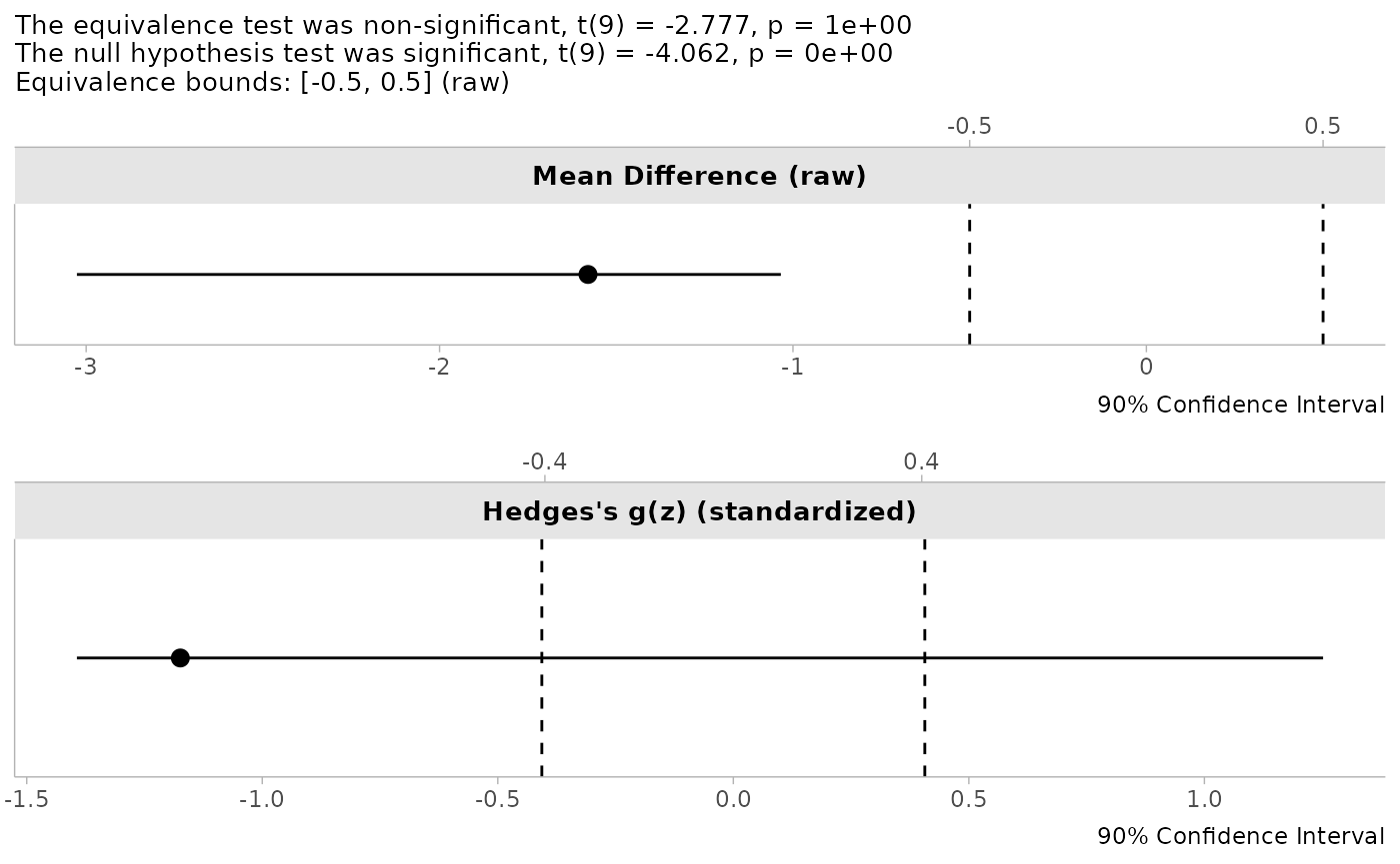

Interpreting Bootstrap TOST Results

When interpreting the results of boot_t_TOST:

The bootstrap p-values (p1 and p2) represent the empirical probability of observing the test statistic or more extreme values under repeated sampling, computed using a method that matches the selected boot_ci
The confidence intervals are derived from the bootstrap distribution using the selected method (studentized, percentile, basic, or BCa)
The distribution plots provide visual insight into the variability of the effect size estimate

Because the p-values and CIs are computed with the same bootstrap method, they will always agree: if the \((1 - 2\alpha)\) CI for the mean difference falls entirely within the equivalence bounds, then both one-sided bootstrap p-values will be significant at level \(\alpha\), and vice versa.

Comparing Bootstrap and Permutation Approaches

To illustrate the similarities and differences between these methods, let’s apply both to the same dataset:

# Same equivalence test using both methods
data('sleep')

# Bootstrap approach
boot_result <- boot_t_test(extra ~ group, 
                           data = sleep,
                           alternative = "equivalence",
                           mu = c(-2, 2),
                           R = 999)

# Permutation approach  
perm_result <- perm_t_test(extra ~ group,
                           data = sleep,
                           alternative = "equivalence", 
                           mu = c(-2, 2),
                           R = 999)

## Note: Number of permutations (R = 999) is less than 1000. Consider increasing R for more stable p-value estimates.

# Compare results
boot_result

## 
##  Bootstrapped Welch Two Sample t-test (studentized)
## 
## data:  extra by group
## t-observed = 0.49465, df = 17.776, p-value = 0.3073
## alternative hypothesis: equivalence
## null values:
## difference in means difference in means 
##                  -2                   2 
## 90 percent confidence interval:
##  -3.0970524 -0.1114282
## sample estimates:
##           mean of group '1'           mean of group '2' 
##                        0.75                        2.33 
## mean difference ('1' - '2') 
##                       -1.58

perm_result

## 
##  Randomization Permutation Welch Two Sample t-test
## 
## data:  extra by group
## t-observed = 0.49465, df = 17.776, p-value = 0.307
## alternative hypothesis: equivalence
## null values:
## difference in means difference in means 
##                  -2                   2 
## 90 percent confidence interval:
##  -3.120 -0.078
## sample estimates:
##           mean of group '1'           mean of group '2' 
##                        0.75                        2.33 
## mean difference ('1' - '2') 
##                       -1.58

Both methods test the same hypothesis and should yield similar conclusions. Key differences to note:

P-values: May differ slightly due to Monte Carlo variability and the different resampling mechanisms
Confidence intervals: Bootstrap uses the resampled effect distribution; permutation uses the percentile method on permuted effects
Exact inference: When sample sizes are small enough, permutation provides exact p-values with no Monte Carlo error

Summary: Choosing Between Methods

Feature	Permutation (`perm_t_test`)	Bootstrap (`boot_t_TOST`/`boot_t_test`)
Resampling type	Without replacement	With replacement
Exact p-values possible	Yes (small samples)	No
Trimmed means support	Yes (`tr` argument)	Yes (`tr` argument in `boot_t_test`)
CI methods	Percentile	Studentized, percentile, basic, BCa
Effect size plots	No	Yes
Best for	Small samples, exact inference	Moderate samples, visualization

For very small samples where exact permutations are feasible, permutation testing is generally preferred because it provides exact p-values (i.e., no need to set a seed). For larger samples or when you want the visualization capabilities of boot_t_TOST or boot_t_test, bootstrapping is a good choice. When outliers are a concern, using perm_t_test with trimming combines the benefits of exact inference with robust location estimation.

Ratio of Difference (Log Transformed)

In many bioequivalence studies, the differences between drugs are compared on the log scale (He et al. 2022). The log scale allows researchers to compare the ratio of two means.

\[ log ( \frac{y}{x} ) = log(y) - log(x) \]

Where:

y and x are the means of the two groups being compared
The transformation converts multiplicative relationships into additive ones

Why Use The Natural Log Transformation?

The United States Food and Drug Administration (FDA)⁴ has stated a rationale for using the log transformed values:

Using logarithmic transformation, the general linear statistical model employed in the analysis of BE data allows inferences about the difference between the two means on the log scale, which can then be retransformed into inferences about the ratio of the two averages (means or medians) on the original scale. Logarithmic transformation thus achieves a general comparison based on the ratio rather than the differences.

Log transformation offers several advantages:

It facilitates the analysis of relative rather than absolute differences
It often makes right-skewed distributions more symmetric
It stabilizes variance when variability increases with the mean
It provides an easy-to-interpret effect size (ratio of means)

In addition, the FDA considers two drugs as bioequivalent when the ratio between x and y is less than 1.25 and greater than 0.8 (1/1.25), which is the default equivalence bound for the log functions.

Applications Beyond Bioequivalence

While log transformation is standard in bioequivalence studies, it’s useful in many other contexts:

Economics: Comparing percentage changes in economic indicators
Environmental science: Analyzing concentration ratios of pollutants
Biology: Examining growth rates or concentration ratios
Medicine: Comparing relative efficacy of treatments
Psychology: Analyzing response time ratios

Consider using log transformation whenever your research question is about relative rather than absolute differences, particularly when the data follow a multiplicative rather than additive pattern.

log_TOST

For example, we could compare whether the cars of different transmissions are “equivalent” with regards to gas mileage. We can use the default equivalence bounds (eqb = 1.25).

log_TOST(
  mpg ~ am,
  data = mtcars
)

## 
## Log-transformed Welch Two Sample t-test
## 
## The equivalence test was non-significant, t(23.96) = -1.363, p = 9.07e-01
## The null hypothesis test was significant, t(23.96) = -3.826, p = 8.19e-04
## NHST: reject null significance hypothesis that the effect is equal to one 
## TOST: don't reject null equivalence hypothesis
## 
## TOST Results 
##                 t    df p.value
## t-test     -3.826 23.96 < 0.001
## TOST Lower -1.363 23.96   0.907
## TOST Upper -6.288 23.96 < 0.001
## 
## Effect Sizes 
##                  Estimate      SE               C.I. Conf. Level
## log(Means Ratio)  -0.3466 0.09061 [-0.5017, -0.1916]         0.9
## Means Ratio        0.7071      NA   [0.6055, 0.8256]         0.9

Note, that the function produces t-tests similar to the t_TOST function, but provides two effect sizes. The means ratio on the log scale (the scale of the test statistics), and the means ratio. The means ratio is missing standard error because the confidence intervals and estimate are simply the log scale results exponentiated.

Interpreting the Means Ratio

When interpreting the means ratio:

A ratio of 1.0 indicates perfect equivalence (no difference)
Ratios > 1.0 indicate that the first group has higher values than the second
Ratios < 1.0 indicate that the first group has lower values than the second

For equivalence testing with the default bounds (0.8, 1.25): - Equivalence is established when the 90% confidence interval for the ratio falls entirely within (0.8, 1.25) - This range corresponds to a difference of ±20% on a relative scale

Bootstrap + Log

However, it has been noted in the statistics literature that t-tests on the logarithmic scale can be biased, and it is recommended that bootstrapped tests be utilized instead. Therefore, the boot_log_TOST function can be utilized to perform a more precise test.

boot_log_TOST(
  mpg ~ am,
  data = mtcars,
  R = 499
)

## 
## Bootstrapped Log Welch Two Sample t-test
## 
## The equivalence test was non-significant, t(23.96) = -1.363, p = 9.62e-01
## The null hypothesis test was significant, t(23.96) = -3.826, p = 0e+00
## NHST: reject null significance hypothesis that the effect is equal to 1 
## TOST: don't reject null equivalence hypothesis
## 
## TOST Results 
##                 t    df p.value
## t-test     -3.826 23.96 < 0.001
## TOST Lower -1.363 23.96   0.962
## TOST Upper -6.288 23.96 < 0.001
## 
## Effect Sizes 
##                  Estimate      SE             C.I. Conf. Level
## log(Means Ratio)  -0.3466 0.08487  [-0.4994, -0.2]         0.9
## Means Ratio        0.7071 0.06060 [0.6069, 0.8187]         0.9
## Note: studentized bootstrap ci method utilized.

The bootstrapped version is particularly recommended when:

Sample sizes are small (n < 30 per group)
Data show notable deviations from log-normality
You want to ensure robust confidence intervals

Like boot_t_TOST, the boot_log_TOST function supports multiple bootstrap CI methods (studentized, percentile, basic, and BCa) via the boot_ci argument, with matched p-values that are guaranteed to agree with the CI. All bootstrap computations are performed on the log scale, then back-transformed.

Standardized, Rank-Based, Effect Sizes: Estimation and Testing

The ses_calc and boot_ses_calc functions calculate rank based standardized effect sizes (rank-biserial correlation, WMW odds, concordance probability, or log-odds) with confidence intervals⁵. As of v0.9.0, ses_calc also supports hypothesis testing directly on the effect size scale.

Available Effect Sizes

Rank-Biserial Correlation

The rank-biserial correlation is a fairly intuitive measure of effect size which has a similar interpretation as the common language effect size (Kerby 2014). However, instead of assuming normality and equal variances, it calculates the number of favorable (positive) and unfavorable (negative) pairs based on their respective ranks.

For the two sample case, the correlation is calculated as the proportion of favorable pairs minus the unfavorable pairs.

\[ r_{biserial} = f_{pairs} - u_{pairs} \]

Where: - \(f_{pairs}\) is the proportion of favorable pairs - \(u_{pairs}\) is the proportion of unfavorable pairs

For the one sample or paired samples cases, the correlation is calculated with ties (values equal to zero) not being dropped. This provides a conservative estimate of the rank biserial correlation.

It is calculated in the following steps wherein \(z\) represents the values or difference between paired observations:

Calculate signed ranks:

\[ r_j = -1 \cdot sign(z_j) \cdot rank(|z_j|) \]

Where: - \(r_j\) is the signed rank for observation \(j\) - \(sign(z_j)\) is the sign of observation \(z_j\) (+1 or -1) - \(rank(|z_j|)\) is the rank of the absolute value of observation \(z_j\)

Calculate the positive and negative sums:

\[ R_{+} = \sum_{1\le i \le n, \space z_i > 0}r_j \]

\[ R_{-} = \sum_{1\le i \le n, \space z_i < 0}r_j \]

Where: - \(R_{+}\) is the sum of ranks for positive observations - \(R_{-}\) is the sum of ranks for negative observations

Determine the smaller of the two rank sums:

\[ T = min(R_{+}, \space R_{-}) \]

\[ S = \begin{cases} -4 & R_{+} \ge R_{-} \\ 4 & R_{+} < R_{-} \end{cases} \]

Where: - \(T\) is the smaller of the two rank sums - \(S\) is a sign factor based on which rank sum is smaller

Calculate rank-biserial correlation:

\[ r_{biserial} = S \cdot | \frac{\frac{T - \frac{(R_{+} + R_{-})}{2}}{n}}{n + 1} | \]

Where: - \(n\) is the number of observations (or pairs) - The final value ranges from -1 to 1

Concordance Probability

The concordance probability (also known as the c-statistic, c-index, or probability of superiority⁶) is converted from the rank-biserial correlation:

\[ c = \frac{(r_{biserial} + 1)}{2} \]

The c-statistic can be interpreted as the probability that a randomly selected observation from one group will be greater than a randomly selected observation from another group. A value of 0.5 indicates no difference between groups, while values approaching 1 indicate perfect separation between groups.

Please note that the c-statistic is equivalent to the area under the receiver operating characteristic curve (AUC) in binary classification contexts. For independent two-sample designs, the c-statistic estimates the same quantity as that produced by brunner_munzel: P(X > Y), the probability that a randomly selected observation from one group exceeds a randomly selected observation from the other. However, for paired samples and one-sample designs, the c-statistic from the Wilcoxon test is based on the difference scores rather than the cross-group comparison, estimating P(Z > 0), where Z (Z = X - Y) represents the paired differences (or deviations from the null value). Additionally, the confidence interval and standard error methods differ between brunner_munzel and the c-statistic reported here.

WMW Odds

The Wilcoxon-Mann-Whitney odds (O’Brien and Castelloe 2006), also known as the “Generalized Odds Ratio”⁷ (Agresti 1980), is calculated by converting the c-statistic:

\[ WMW_{odds} = e^{logit(c)} \]

Where \(logit(c) = \ln\frac{c}{1-c}\)

The WMW odds can be interpreted similarly to a traditional odds ratio, representing the odds that an observation from one group is greater than an observation from another group.

Guidelines for Selecting Effect Size Measures

Rank-biserial correlation ("rb") is useful when you want a correlation-like measure that’s easily interpretable and comparable to other correlation coefficients.
Concordance probability ("cstat") is beneficial when you want to express the effect in terms of probability, making it accessible to non-statisticians.
WMW odds ("odds") is helpful when you want to express the effect in terms familiar to those who work with odds ratios in logistic regression or epidemiology, or interpreting probabilities as odds (e.g., betting and prediction markets).
WMW log-odds ("logodds") the log-odds can be helpful because you could interpret them as a percent difference/change in the odds of stochastic superiority. E.g., if the WMW log-odds were 0.10 then you could say “X increases the odds of superiority by approximately 10% over Y”.

Confidence Interval Methods

As of v0.9.0, the TOSTER package defaults to the score method (se_method = "score") for computing standard errors and confidence intervals for all SES functions (see function documentation for more information). There is also the Agresti method. This method uses placement-based variance estimation and conducts inference on the log-odds scale, which performs fairly well when the degree of seperation between groups is not high. Results are back-transformed to the requested effect size scale for reporting. The Fisher z-transformation method (se_method = "fisher") remains available as a legacy option. This was the default in earlier versions of the package and is documented below for reference.

Fisher z-Transformation (Legacy Method)

The Fisher approximation calculates confidence intervals by first computing a standard error, then transforming to a Fisher z-scale for interval construction.

For paired samples, or one sample, the standard error is calculated as:

\[ SE_r = \sqrt{ \frac {(2 \cdot nd^3 + 3 \cdot nd^2 + nd) / 6} {(nd^2 + nd) / 2} } \]

wherein, nd represents the total number of observations (or pairs).

For independent samples, the standard error is:

\[ SE_r = \sqrt{\frac {(n1 + n2 + 1)} { (3 \cdot n1 \cdot n2)}} \]

Where:

\(n1\) and \(n2\) are the sample sizes of the two groups

The confidence intervals are then calculated by transforming the estimate:

\[ r_z = atanh(r_{biserial}) \]

Then the confidence interval can be calculated and back transformed:

\[ r_{CI} = tanh(r_z \pm Z_{(1 - \alpha / 2)} \cdot SE_r) \]

Where:

\(Z_{(1 - \alpha / 2)}\) is the critical value from the standard normal distribution
\(\alpha\) is the significance level (typically 0.05)

Effect Size Estimation

The interface is similar to wilcox_TOST, but rather than setting equivalence bounds on the raw scale, ses_calc works directly with the standardized effect size. By default (with alternative = "none"), it returns an effect size estimate and confidence interval with no hypothesis test:

# Rank-biserial correlation for paired data
ses_calc(x = sleep$extra[sleep$group == 1],
         y = sleep$extra[sleep$group == 2],
         paired = TRUE,
         ses = "rb")

## 
##  Paired Sample Rank-Biserial Correlation estimate with CI
## 
## data:  sleep$extra[sleep$group == 1] and sleep$extra[sleep$group == 2]
## 
## alternative hypothesis: none
## 95 percent confidence interval:
##  -1.0000000 -0.2989533
## sample estimates:
## P(X - Y>0) - P(X - Y<0) 
##                      -1

Hypothesis Testing with `ses_calc`

As of v0.9.0, ses_calc supports hypothesis testing directly on the effect size scale by setting the alternative argument. This allows you to test whether a non-parametric effect size differs from a specified value, or whether it falls within equivalence bounds, without needing the raw-scale equivalence bounds required by wilcox_TOST.

# Two-sided test: does the rank-biserial differ from 0?
ses_calc(x = sleep$extra[sleep$group == 1],
         y = sleep$extra[sleep$group == 2],
         paired = TRUE,
         ses = "rb",
         alternative = "two.sided")

## 
##  Paired Sample Rank-Biserial Correlation test
## 
## data:  sleep$extra[sleep$group == 1] and sleep$extra[sleep$group == 2]
## z = -2.6679, p-value = 0.007632
## alternative hypothesis: true P(X - Y>0) - P(X - Y<0) is not equal to 0
## 95 percent confidence interval:
##  -1.0000000 -0.2989533
## sample estimates:
## P(X - Y>0) - P(X - Y<0) 
##                      -1

Equivalence Testing on the Effect Size Scale

One advantage of testing directly on the effect size scale is that equivalence bounds have a more intuitive interpretation much like the brunner_munzel test. In fact, you should probably use the brunner_munzel approach for the two-sample case, but the ses_calc functions allow for comparison of paired samples and one-sample case in what that the Brunner-Munzel approach does not allow. Rather than specifying bounds in raw units (which depends on the location-shift assumption), you can specify bounds directly in terms of the effect size:

# Equivalence test: is the rank-biserial within [-0.3, 0.3]?
ses_calc(x = sleep$extra[sleep$group == 1],
         y = sleep$extra[sleep$group == 2],
         paired = TRUE,
         ses = "rb",
         alternative = "equivalence",
         null.value = c(-0.3, 0.3))

## 
##  Paired Sample Rank-Biserial Correlation test
## 
## data:  sleep$extra[sleep$group == 1] and sleep$extra[sleep$group == 2]
## z = -1.9577, p-value = 0.9749
## alternative hypothesis: equivalence
## null values:
## lower bound upper bound 
##        -0.3         0.3 
## 90 percent confidence interval:
##  -1.0000000 -0.4491576
## sample estimates:
## P(X - Y>0) - P(X - Y<0) 
##                      -1

When using ses_calc for hypothesis testing, the se_method argument (described in the Confidence Interval Methods section above) also controls how test statistics are computed. The default Agresti method conducts tests on the log-odds scale, while the Fisher method uses z-transformation. See above for details.

# Using the Agresti method (default) with WMW odds
ses_calc(formula = extra ~ group,
         data = sleep,
         ses = "odds",
         alternative = "two.sided")

## 
##  Two Sample WMW Odds test
## 
## data:  extra by group
## z = -1.8541, p-value = 0.06372
## alternative hypothesis: true odds(P('1'>'2') + .5*P('1'='2')) is not equal to 1
## 95 percent confidence interval:
##  0.1185837 1.0570531
## sample estimates:
## odds(P('1'>'2') + .5*P('1'='2')) 
##                        0.3422819

Bootstrap Based Effect Size Testing with `boot_ses_calc`

When asymptotic approximations may be unreliable, particularly with small samples, boot_ses_calc uses bootstrapping to estimate the sampling distribution of the effect size. Note that bootstrap methods cannot work in situations where there is complete separation between groups (e.g., all values in one group are higher than the other), which can occur with small samples and large effects.

Like the other bootstrap functions in the package, boot_ses_calc supports multiple bootstrap CI methods (studentized, percentile, basic, and BCa) via boot_ci, with p-values matched to the selected CI method for guaranteed CI/p-value agreement. All bootstrap computations are performed on a working scale then back-transformed to the requested effect size scale.

Summary Comparison of Robust TOST Methods

Method	Estimand	Key Advantages	Limitations	Best Use Cases
Wilcoxon-Mann-Whitney	Pseudo-median of pairwise differences (two-sample) or Walsh averages (paired)	Simple, widely accepted	Estimand \(\neq\) mean or median difference without location shift assumption	Ordinal data; legacy analyses
Brunner-Munzel	\(P(X > Y) + 0.5 \cdot P(X = Y)\)	Clear interpretation, robust to heteroscedasticity	Not a location measure	Stochastic superiority/dominance
Hodges-Lehmann	Same as WMW, with Fried-Dehling inference	Robust location, outlier resistant	Same estimand caveats as WMW; inference differs from `wilcox_TOST`	Robust location shift testing with outlier protection
Permutation t-test	\(\mu_X - \mu_Y\) (or trimmed means if `tr` > 0)	Exact p-values, direct mean comparison	Outlier sensitive (unless trimmed)	Mean differences with small samples
Bootstrap t-test	\(\mu_X - \mu_Y\)	Flexible, visualization	Results vary between runs	Mean differences with moderate samples
Log-Transformed	\(\log(\mu_Y / \mu_X)\)	Ratio-based, stabilizes variance	Requires positive data	Bioequivalence, ratio comparisons
*SES calc	Non-parametric effect sizes (rank-biserial, concordance, odds)	Tests directly on effect size scale	Requires large samples (asymptotic) or many replicates	Non-parametric effect size testing

Conclusion

The robust TOST procedures provided in the TOSTER package offer reliable alternatives to standard t-test based equivalence testing when data violate typical assumptions. By selecting the appropriate robust method for your specific data characteristics and research question, you can ensure more valid statistical inferences about equivalence or minimal effects.

Remember that no single method is universally superior — the choice depends on your data structure, sample size, and specific research question. When in doubt, running multiple approaches and comparing results can provide valuable insights into the robustness of your conclusions.

References

Agresti, Alan. 1980. “Generalized Odds Ratios for Ordinal Data.” Biometrics, 59–67. https://doi.org/10.2307/2530495.

Brunner, Edgar, and Ullrich Munzel. 2000. “The Nonparametric Behrens-Fisher Problem: Asymptotic Theory and a Small-Sample Approximation.” Biometrical Journal 42 (1): 17–25. https://doi.org/10.1002/(sici)1521-4036(200001)42:1<17::aid-bimj17>3.0.co;2-u.

Chung, EunYi, and Joseph P. Romano. 2013. “Exact and Asymptotically Robust Permutation Tests.” The Annals of Statistics 41 (2). https://doi.org/10.1214/13-aos1090.

Divine, George W, H James Norton, Anna E Barón, and Elizabeth Juarez-Colunga. 2018. “The Wilcoxon–Mann–Whitney Procedure Fails as a Test of Medians.” The American Statistician 72 (3): 278–86. https://doi.org/10.1080/00031305.2017.1305291.

Efron, Bradley, and Robert J. Tibshirani. 1993. An Introduction to the Bootstrap. Monographs on Statistics and Applied Probability 57. Boca Raton, Florida, USA: Chapman & Hall/CRC.

Fried, Roland, and Herold Dehling. 2011. “Robust Nonparametric Tests for the Two-Sample Location Problem.” Stat. Methods Appt. 20 (4): 409–22.

He, Y, Y Deng, C You, and X H Zhou. 2022. “Equivalence Tests for Ratio of Means in Bioequivalence Studies Under Crossover Designs.” Statistical Methods in Medical Research, 09622802221093721. https://doi.org/10.1177/09622802221093721.

Hodges, Joseph L, and Erich L Lehmann. 1963. “Estimates of Location Based on Rank Tests.” The Annals of Mathematical Statistics 34 (2): 598–611. https://doi.org/10.1214/aoms/1177704172.

Janssen, Arnold. 1997. “Studentized Permutation Tests for Non-i.i.d. Hypotheses and the Generalized Behrens-Fisher Problem.” Statistics and Probability Letters 36 (1): 9–21. https://doi.org/10.1016/s0167-7152(97)00043-6.

Karch, Julian D. 2021. “Psychologists Should Use Brunner-Munzel’s Instead of Mann-Whitney’s Test as the Default Nonparametric Procedure.” Advances in Methods and Practices in Psychological Science 4 (2): 251524592199960. https://doi.org/10.1177/2515245921999602.

Kerby, Dave S. 2014. “The Simple Difference Formula: An Approach to Teaching Nonparametric Correlation.” Comprehensive Psychology 3 (January): 11.IT.3.1. https://doi.org/10.2466/11.it.3.1.

Munzel, Ullrich, and Dieter Hauschke. 2003. “A Nonparametric Test for Proving Noninferiority in Clinical Trials with Ordered Categorical Data.” Pharm. Stat. 2 (1): 31–37.

Neubert, Karin, and Edgar Brunner. 2007. “A Studentized Permutation Test for the Non-Parametric Behrensfisher Problem.” Computational Statistics and Data Analysis 51 (10): 5192–5204. https://doi.org/10.1016/j.csda.2006.05.024.

O’Brien, Ralph G, and John Castelloe. 2006. “Exploiting the Link Between the Wilcoxon-Mann-Whitney Test and a Simple Odds Statistic,” 209–31.

Phipson, Belinda, and Gordon K Smyth. 2010. “Permutation p-Values Should Never Be Zero: Calculating Exact p-Values When Permutations Are Randomly Drawn.” Statistical Applications in Genetics and Molecular Biology 9 (1). https://doi.org/10.2202/1544-6115.1585.

Aaron R. Caldwell

2026-03-16

Introduction to Robust TOST Methods

Choosing by Estimand

When to Use Robust TOST Methods

Wilcoxon-Mann-Whitney TOST

Why WMW Tests Can Be Misleading

What WMW actually tests

Counterexamples

The problem for equivalence testing

What to use instead

Key Features and Usage

Understanding the Equivalence Bounds (eqb)

Interpreting the Results

Standardized Effect Sizes

Interface with wilcox.test

Brunner-Munzel Test

Overview and Advantages

Basics of the Calculative Approach

Test Methods

Examples

Basic Two-Sample Test

Logit Transformation for Range-Preserving CIs

Equivalence Testing

Minimal Effect Testing

Paired Samples

Testing Against a Non-Standard Null

Interpreting Brunner-Munzel Results

Choosing the Right Test Method

Non-Inferiority Testing

Hodges-Lehmann Estimator and Test

Why Use the Hodges-Lehmann Estimator?

Estimators

Interpreting the Estimand

Test Methods

Examples

Basic Two-Sample Test

Permutation-Based Test

Equivalence Testing

Paired Samples

Minimal Effect Testing

Choosing the Right Approach

Resampling Methods: Bootstrapping and Permutation

Conceptual Overview

When to Use Each Method

Permutation t-test

Permutation Procedure

Two-Sample Permutation Algorithm

Welch Variant (var.equal = FALSE)

Pooled Variance Variant (var.equal = TRUE)

Yuen Variant (tr > 0)

Studentized Permutation: The perm_se Argument

Combining Permutation with Trimmed Means

Example: Basic Permutation Test

Example: Permutation Test with Trimming

Example: Equivalence Testing with Permutation

Exact vs. Monte Carlo Permutations

Bootstrap t-test

Advantages of Bootstrapping

Bootstrap Algorithm (Two-Sample Case)

Bootstrap CI Methods and P-value Consistency

Choosing the Number of Bootstrap Replications

Example

Interpreting Bootstrap TOST Results

Comparing Bootstrap and Permutation Approaches

Summary: Choosing Between Methods

Ratio of Difference (Log Transformed)

Why Use The Natural Log Transformation?

Applications Beyond Bioequivalence

log_TOST

Interpreting the Means Ratio

Bootstrap + Log

Standardized, Rank-Based, Effect Sizes: Estimation and Testing

Available Effect Sizes

Rank-Biserial Correlation

Concordance Probability

WMW Odds

Guidelines for Selecting Effect Size Measures

Confidence Interval Methods

Understanding the Equivalence Bounds (`eqb`)

Interface with `wilcox.test`

Studentized Permutation: The `perm_se` Argument

Hypothesis Testing with `ses_calc`

Bootstrap Based Effect Size Testing with `boot_ses_calc`