Standardized Mean Differences
The calculation of Cohen’s d type effect sizes
Aaron R. Caldwell
2026-04-17
SMD_calcs.RmdThe calculation of standardized mean differences (SMDs) can be helpful in interpreting data and are essential for meta-analysis. In psychology, effect sizes are very often reported as an SMD rather than raw units (though either is fine: see Caldwell and Vigotsky (2020)). In most papers the SMD is reported as Cohen’s d1. The simplest form involves reporting the mean difference (or mean in the case of a one-sample test) divided by the standard deviation.
\[ Cohen's \space d = \frac{Mean}{SD} = SMD \]
However, two major problems arise: bias and the calculation of the denominator. First, the Cohen’s d calculation is biased (meaning the effect is inflated), and a bias correction (often referred to as Hedges’ g) is applied to provide an unbiased estimate. Second, the denominator can influence the estimate of the SMD, and there are a multitude of choices for how to calculate the denominator. To make matters worse, the calculation (in most cases an approximation) of the confidence intervals involves the noncentral t distribution. This requires calculating a non-centrality parameter (lambda: \(\lambda\)), degrees of freedom (\(df\)), or even the standard error (sigma: \(\sigma\)) for the SMD. None of these are easy to determine and these calculations are hotly debated in the statistics literature (Cousineau and Goulet-Pelletier 2021).
In this package we originally opted to make the default SMD
confidence intervals as the formulation outlined by Goulet-Pelletier and Cousineau (2018). We found that that these
calculations were simple to implement and provided fairly accurate
coverage for the confidence intervals for any type of SMD (independent,
paired, or one sample). However, even the authors have outlined some
issues with the method in a newer publication (Cousineau and Goulet-Pelletier
2021). Other packages, such as MOTE (Buchanan et al. 2019)
or effectsize (Ben-Shachar, Lüdecke, and Makowski
2020), use a simpler formulation of the noncentral
t-distribution (nct). The default option in the package is the nct type
of confidence intervals. We have created an argument for all TOST
functions (tsum_TOST and t_TOST) named
smd_ci which allow the user to specify “goulet” (for the
Cousineau and Goulet-Pelletier (2021) method), “nct” (this will
approximately match the results of Buchanan et
al. (2019) and Ben-Shachar, Lüdecke, and Makowski (2020)), “t” (central t method), or “z”
(normal method). We would recommend using “nct” as the default for any
analysis but as Viechtbauer (2007) points out the
approximate methods usually suffice. It is important to remember that
all of these methods are only approximations of confidence
intervals (of varying degrees of quality) and therefore should be
interpreted with caution.
It is my belief that SMDs provide another interesting quantitative
effect size description, but have dubious and limited inferential
utility2.
You may disagree, and if you are basing your inferences on the SMD, and
the associated confidence intervals, we recommend you go with a
bootstrapping approach (see
boot_smd_calc Kirby and Gerlanc
2013) as it is a more robust option.
In this section we will detail on the calculations that are involved in calculating the SMD, their associated degrees of freedom, non-centrality parameter, and variance. If these SMDs are being reported in a scientific manuscript, we strongly recommend that the formulas for the SMDs you report be included in the methods section.
Bias Correction (Hedges)
For all SMD calculative approaches the bias correction was calculated as the following:
\[ J = \frac{\Gamma(\frac{df}{2})}{\sqrt{\frac{df}{2}} \cdot \Gamma(\frac{df-1}{2})} \]
The correction factor3 is calculated in R as the following:
J <- exp ( lgamma(df/2) - log(sqrt(df/2)) - lgamma((df-1)/2) )Hedges g (bias corrected SMD) can then be calculated by multiplying the SMD by J
\[ g = SMD \cdot J \] When the bias correction is not applied, J is equal to 1.
Independent Samples
For independent samples there are three calculative approaches
supported by TOSTER. One the denominator is the pooled
standard deviation (Cohen’s d), the average standard deviation (Cohen’s
d(av)), and the standard deviation of the control group (Glass’s \(\Delta\)). Currently, the d or d(av) is
selected by whether or not variances are assumed to be equal. If the
variances are not assumed to be equal then Cohen’s d(av) will be
returned, and if variances are assumed to be equal then Cohen’s d is
returned. Glass’s delta can be selected by setting the
glass argument to “glass1” or “glass2”.
Variances Assumed Unequal: Cohen’s d(av)
For this calculation, the denominator is simply the square root of the average variance.
\[ s_{av} = \sqrt \frac {s_{1}^2 + s_{2}^2}{2} \]
The SMD, Cohen’s d(av), is then calculated as the following:
\[ d_{av} = \frac {\bar{x}_1 - \bar{x}_2} {s_{av}} \]
Note: the x with the bar above it (pronounced as “x-bar”) refers the the means of group 1 and 2 respectively.
The degrees of freedom for Cohen’s d(av), derived from Delacre et al. (2021), is the following:
\[ df = \frac{(n_1-1)(n_2-1)(s_1^2+s_2^2)^2}{(n_2-1) \cdot s_1^4+(n_1-1) \cdot s_2^4} \]
The non-centrality parameter (\(\lambda\)) is calculated as the following:
- Under the Cousineau and Goulet-Pelletier (2021) method
(
smd_ci = "goulet"):
\[ \lambda = d_{av} \times \sqrt{\frac{n_1 \cdot n_2(\sigma^2_1+\sigma^2_2)}{2 \cdot (n_2 \cdot \sigma^2_1+n_1 \cdot \sigma^2_2)}} \]
- Under all other methods (nct, t, or z):
\[ \lambda = \frac{2 \cdot (n_2 \cdot \sigma_1^2 + n_1 \cdot \sigma_2^2)} {n_1 \cdot n_2 \cdot (\sigma_1^2 + \sigma_2^2)} \] The standard error (\(\sigma\)) of Cohen’s d(av) is calculated as the following from Bonett (2009)4:
\[ \sigma_{SMD} = \sqrt{d^2 \cdot (\frac{s_1^4}{n_1-1}+\frac{s_2^4}{n_2-1}) \div 8 \cdot s_{av}^4 + (\frac{s_1^2}{n_1-1}+\frac{s_2^2}{n_2-1}) \div s_{av}^2} \]
Variances Assumed Equal: Cohen’s d
For this calculation, the denominator is simply the pooled standard deviation.
\[ s_{p} = \sqrt \frac {(n_{1} - 1)s_{1}^2 + (n_{2} - 1)s_{2}^2}{n_{1} + n_{2} - 2} \]
\[ d = \frac {\bar{x}_1 - \bar{x}_2} {s_{p}} \]
The degrees of freedom for Cohen’s d is the following:
\[ df = n_1 + n_2 - 2 \]
The non-centrality parameter (\(\lambda\)) is calculated as the following:
- Under the Cousineau and Goulet-Pelletier (2021) method
(
smd_ci = "goulet"):
\[ \lambda = d \cdot \sqrt \frac{\tilde n}{2} \]
wherein, \(\tilde n\) is the harmonic mean of the 2 sample sizes which is calculated as the following:
\[ \tilde n = \frac{2 \cdot n_1 \cdot n_2}{n_1 + n_2} \]
- Under all other methods (nct, t, or z):
\[ \lambda = \frac{1}{n_1} +\frac{1}{n_2} \]
The standard error (\(\sigma\)) of Cohen’s d is calculated as the following:
- Under the Cousineau and Goulet-Pelletier (2021) method
(
smd_ci = "goulet"):
\[ \sigma_{SMD} = \sqrt{\frac{df}{df-2} \cdot \frac{2}{\tilde n} (1+d^2 \cdot \frac{\tilde n}{2}) -\frac{d^2}{J}} \]
- Under all other methods (nct, t, or z) it is calculated using the “unbiased” estimate from Viechtbauer (2007) (table 1; equation 26)5:
\[ \sigma_{SMD} = \sqrt{\frac{1}{n_1} + \frac{1}{n_2} + (1 - \frac{df-2}{df \cdot J^2}) \cdot d_s^2} \]
Glass’s Delta
For this calculation, the denominator is simply the standard
deviation of one of the groups (x for
glass = "glass1", or y for
glass = "glass2".
\[ s_{c} = SD_{control \space group} \]
\[ d = \frac {\bar{x}_1 - \bar{x}_2} {s_{c}} \]
The degrees of freedom for Glass’s delta is the following:
\[ df = n_c - 1 \]
The non-centrality parameter (\(\lambda\)) is calculated as the following:
- Under the Cousineau and Goulet-Pelletier (2021) method
(
smd_ci = "goulet"):
\[ \lambda = d \cdot \sqrt \frac{\tilde n}{2} \]
wherein, \(\tilde n\) is the harmonic mean of the 2 sample sizes which is calculated as the following:
\[ \tilde n = \frac{2 \cdot n_1 \cdot n_2}{n_1 + n_2} \]
- Under all other methods (nct, t, or z):
\[ \lambda = \frac{1}{n_T} + \frac{s_c^2}{n_c \cdot s_c^2} \]
The standard error (\(\sigma\)) of Glass’s delta is calculated as the following:
- Under the Cousineau and Goulet-Pelletier (2021) method
(
smd_ci = "goulet"):
\[ \sigma_{SMD} = \sqrt{\frac{df}{df-2} \cdot \frac{2}{\tilde n} (1+d^2 \cdot \frac{\tilde n}{2}) -\frac{d^2}{J}} \]
\[ \sigma_{SMD} = \sqrt{\frac{s_e^2 \div s_c^2}{n_e-1}+ \frac{1}{n_c-1}+ \frac{d^2}{2 \cdot (n_c-1)}} \]
Paired Samples
For paired samples there are two calculative approaches supported by
TOSTER. One the denominator is the standard deviation of
the change score (Cohen’s d(z)), the correlation corrected effect size
(Cohen’s d(rm)), and the standard deviation of the control condition
(Glass’s \(\Delta\)). Currently, the
choice is made by the function based on whether or not the user sets
rm_correction to TRUE. If rm_correction is set
to t TRUE then Cohen’s d(rm) will be returned, and otherwise Cohen’s
d(z) is returned. This can be overridden and Glass’s delta is returned
if the glass argument is set to “glass1” or “glass2”.
Cohen’s d(z): Change Scores
For this calculation, the denominator is the standard deviation of the difference scores which can be calculated from the standard deviations of the samples and the correlation between the paired samples.
\[ s_{diff} = \sqrt{sd_1^2 + sd_2^2 - 2 \cdot r_{12} \cdot sd_1 \cdot sd_2} \]
The SMD, Cohen’s d(z), is then calculated as the following:
\[ d_{z} = \frac {\bar{x}_1 - \bar{x}_2} {s_{diff}} \]
The degrees of freedom for Cohen’s d(z) is the following:
- Under the Cousineau and Goulet-Pelletier (2021) method
(
smd_ci = "goulet"):
\[ df = 2 \cdot (N_{pairs}-1) \]
- Under all other methods (nct, t, or z):
\[ df = N - 1 \]
The non-centrality parameter (\(\lambda\)) is calculated as the following:
- Under the Cousineau and Goulet-Pelletier (2021) method
(
smd_ci = "goulet"):
\[ \lambda = d_{z} \cdot \sqrt \frac{N_{pairs}}{2 \cdot (1-r_{12})} \]
- Under all other methods (nct, t, or z):
\[ \lambda = \frac{1}{n} \]
The standard error (\(\sigma\)) of Cohen’s d(z) is calculated as the following:
- Under the Cousineau and Goulet-Pelletier (2021) method
(
smd_ci = "goulet"):
\[ \sigma_{SMD} = \sqrt{\frac{df}{df-2} \cdot \frac{2 \cdot (1-r_{12})}{n} \cdot (1+d^2 \cdot \frac{n}{2 \cdot (1-r_{12})}) -\frac{d^2}{J^2}} \space \times \space \sqrt {2 \cdot (1-r_{12})} \]
- Under all other methods (nct, t, or z) it calculated using the “unbiased” estimate from Viechtbauer (2007) (table 1; equation 26)7:
\[ \sigma_{SMD} = \sqrt{\frac{1}{N} + (1 - \frac{df-2}{df \cdot J^2}) \cdot d_z^2} \]
Cohen’s d(rm): Correlation Corrected
For this calculation, the same values for the same calculations above is adjusted for the correlation between measures. As Goulet-Pelletier and Cousineau (2018) mention, this is useful for when effect sizes are being compared for studies that involve between and within subjects designs.
First, the standard deviation of the difference scores are calculated
\[ s_{diff} = \sqrt{sd_1^2 + sd_2^2 - 2 \cdot r_{12} \cdot sd_1 \cdot sd_2} \]
The SMD, Cohen’s d(rm), is then calculated with a small change to the denominator8:
\[ d_{rm} = \frac {\bar{x}_1 - \bar{x}_2}{s_{diff}} \cdot \sqrt {2 \cdot (1-r_{12})} \]
The degrees of freedom for Cohen’s d(rm) is the following:
- Under the Cousineau and Goulet-Pelletier (2021) method
(
smd_ci = "goulet"):
\[ df = 2 \cdot (N_{pairs}-1) \]
- Under all other methods (nct, t, or z):
\[ df = N - 1 \]
The non-centrality parameter (\(\lambda\)) is calculated as the following:
- Under the Cousineau and Goulet-Pelletier (2021) method
(
smd_ci = "goulet"):
\[ \lambda = d_{rm} \cdot \sqrt \frac{N_{pairs}}{2 \cdot (1-r_{12})} \]
- Under all other methods (nct, t, or z):
\[ \lambda = \frac{1}{n} \]
The standard error (\(\sigma\)) of Cohen’s d(rm) is calculated as the following:
\[ \sigma_{SMD} = \sqrt{\frac{df}{df-2} \cdot \frac{2 \cdot (1-r_{12})}{n} \cdot (1+d_{rm}^2 \cdot \frac{n}{2 \cdot (1-r_{12})}) -\frac{d_{rm}^2}{J^2}} \]
Glass’s Delta
For this calculation, the denominator is simply the standard
deviation of one of the groups (x for
glass = "glass1", or y for
glass = "glass2".
\[ s_{c} = SD_{control \space condition} \]
\[ d = \frac {\bar{x}_1 - \bar{x}_2} {s_{c}} \]
The degrees of freedom for Glass’s delta is the following:
- Under the Cousineau and Goulet-Pelletier (2021) method
(
smd_ci = "goulet"):
\[ df = 2 \cdot N - 1 \]
- Under all other methods (nct, t, or z):
\[ df = N - 1 \]
The non-centrality parameter (\(\lambda\)) is calculated as the following:
- Under the Cousineau and Goulet-Pelletier (2021) method
(
smd_ci = "goulet"):
\[ \lambda = d \cdot \sqrt{\frac{N}{2 \cdot (1 - r_{12})}} \]
- Under all other methods (nct, t, or z):
\[ \lambda = \frac{1}{N} \]
The standard error (\(\sigma\)) of Glass’s delta is calculated as the following derived9 from Bonett (2008):
\[ \sigma_{SMD} = \sqrt{\frac{s_{diff}^2}{s_c^2 \cdot df} + \frac{d^2}{2 \cdot df}} \]
One Sample
For a one-sample situation, the calculations are very straight forward
For this calculation, the denominator is simply the standard deviation of the sample.
\[ s={\sqrt {{\frac {1}{N-1}}\sum _{i=1}^{N}\left(x_{i}-{\bar {x}}\right)^{2}}} \]
The SMD is then the mean of X divided by the standard deviation.
\[ d = \frac {\bar{x}} {s} \]
The degrees of freedom for Cohen’s d is the following:
\[ df = N - 1 \]
The non-centrality parameter (\(\lambda\)) is calculated as the following:
\[ \lambda = d \cdot \sqrt N \]
The standard error (\(\sigma\)) of Cohen’s d is calculated as the following:
- Under the Cousineau and Goulet-Pelletier (2021) method
(
smd_ci = "goulet"):
\[ \sigma_{SMD} = \sqrt{\frac{df}{df-2} \cdot \frac{1}{N} (1+d^2 \cdot N) -\frac{d^2}{J^2}} \]
- Under all other methods (nct, t, or z):
\[ \sigma_{SMD} = \sqrt{\frac{1}{n} + \frac{d^2}{(2 \cdot n)}} \]
Confidence Intervals
For the SMDs calculated in this package we use the non-central
t method, those outlined by Goulet-Pelletier and Cousineau (2018), and approximate methods using
the t and normal distributions. These calculations are only
approximations and newer formulations may provide better coverage (e.g., Cousineau and
Goulet-Pelletier 2021). In any case, if the calculation of
confidence intervals for SMDs is of the utmost importance then I would
strongly recommend using bootstrapping techniques rather than any of
these approximations whenever possible (Kirby and Gerlanc 2013), and these
methods are available in the boot_smd_calc function.
The calculations of the confidence intervals for the
goulet and nct methods involve a two step
process: 1) using the noncentral t-distribution to calculate
the lower and upper bounds of \(\lambda\), and 2) transforming this back to
the effect size estimate. These noncentrality methods are not without
their detractors (Spanos 2021). The normal and
t methods are much simpler and less computationally intensive,
but may have varying levels of accuracy (see Viechtbauer 2007 for more
details).
Cousineau and Goulet-Pelletier (2021) Method (smd_ci = “goulet”)
Calculate confidence intervals around \(\lambda\).
\[ t_L = t_{(1/2-(1-\alpha)/2,\space df, \space \lambda)} \\ t_U = t_{(1/2+(1-\alpha)/2,\space df, \space \lambda)} \]
Then transform back to the SMD.
\[ d_L = \frac{t_L}{\lambda} \cdot d \\ d_U = \frac{t_U}{\lambda} \cdot d \]
The non-central t-method (smd_ci = “nct”)
This method is commonly reported in the literature and in other R
packages (e.g., effectsize). However, it is not without
criticism (Spanos
2021; Viechtbauer
2007).
In thise method, you calculate the non-centrality parameters necessary to form confidence intervals wherein the observed t-statistic (\(t_{obs}\))is utilized.
\[ t_L = t_{(1-alpha,\space df, \space t_{obs})} \\ t_U = t_{(alpha,\space df, \space t_{obs})} \] The confidence intervals can then be constructed using the non-centrality parameter and the bias correction.
\[ d_L = t_L \cdot \sqrt{\lambda} \cdot J \\ d_U = t_U \cdot \sqrt{\lambda} \cdot J \]
Central t-method
This is less commonly used though it might perform alright in some scenarios, and as Bonett (2008) and Viechtbauer (2007) report it might perform adequately under with an adequately large sample size.
The limits of the t-distribution at the given alpha-level and degrees
of freedom (qt(1-alpha,df)) are multiplied by the standard
error of the calculated SMD.
\[ CI = SMD \space \pm \space t_{(1-\alpha,df)} \cdot \sigma_{SMD} \]
Normal method
This method will often be the most liberal estimate for the confidence interval. But as Bonett (2008) and Viechtbauer (2007) report, it might perform adequately under with an adequately large sample size. The use of the normal distribution can be justified by the fact that SMDs are asympototically normal.
The limits of the z-distribution at the given alpha-level
(qnorm(1-alpha)) are multiplied by the standard error of
the calculated SMD.
\[ CI = SMD \space \pm \space z_{(1-\alpha)} \cdot \sigma_{SMD} \]
Just Estimate the SMD
It was requested that a function be provided that only calculates the
SMD. Therefore, I created the smd_calc and
boot_smd_calc functions10. The interface is almost the same as
t_TOST but you don’t set an equivalence bound.
# For paired tests, use separate vectors
smd_calc(x = sleep$extra[sleep$group == 1],
         y = sleep$extra[sleep$group == 2],
         paired = TRUE,
         smd_ci = "nct",
         bias_correction = F)
#>
#>  Paired Sample Standardized Mean Difference (SMD; Cohen's
#>  d[z]=(x-y)/SD_z)
#>
#> data:  sleep$extra[sleep$group == 1] and sleep$extra[sleep$group == 2]
#>
#> alternative hypothesis: none
#> 95 percent confidence interval:
#>  -2.1180165 -0.4146278
#> sample estimates:
#> SMD (d[z])
#>  -1.284558

# Setting bootstrap replications low to
## reduce compiling time of vignette
boot_smd_calc(x = sleep$extra[sleep$group == 1],
              y = sleep$extra[sleep$group == 2],
         R = 199,
         paired = TRUE,
         boot_ci = "stud",
         bias_correction = F)
#>
#>  Paired Sample bootstrapped Standardized Mean Difference (SMD; Cohen's
#>  d[z]=(x-y)/SD_z)
#>
#> data:  sleep$extra[sleep$group == 1] and sleep$extra[sleep$group == 2]
#>
#> alternative hypothesis: none
#> 95 percent confidence interval:
#>  -1.696643  2.584537
#> sample estimates:
#> SMD (d[z])
#>  -1.284558
If you have a hypothesis that is specifically about the SMD then you
can use boot_smd_calc to directly test it by using the
null.value and alternative value arguments.
For example, you might have a hypothesis of equivalence regarding the
SMD, and therefore you could set null.value = c(-0.5,0.5)
if you hypothesize that the SMD is between 0.5 and -0.5 and
alternative = "equivalent" to directly test this
hypothesis.
boot_smd_calc(x = sleep$extra[sleep$group == 1],
              y = sleep$extra[sleep$group == 2],
         R = 199,
         paired = TRUE,
         boot_ci = "stud",
         bias_correction = TRUE,
         null.value = c(-0.5,0.5),
         alternative = "equ")
#>
#>  Paired Sample bootstrapped Standardized Mean Difference (SMD; Hedges's
#>  g[z]=(x-y)/SD_z)
#>
#> data:  sleep$extra[sleep$group == 1] and sleep$extra[sleep$group == 2]
#> z-observed = -2.5211, p-value = 0.7638
#> alternative hypothesis: equivalence
#> null values:
#> lower bound upper bound
#>        -0.5         0.5
#> 90 percent confidence interval:
#>  -1.4018610  0.7932114
#> sample estimates:
#> SMD (g[z])
#>  -1.173925
Plotting SMDs
Sometimes you may take a different approach to calculating the SMD,
or you may only have the summary statistics from another study. For this
reason, I have included a way to plot the SMD based on just three
values: the estimate of the SMD, the degrees of freedom, and the
non-centrality parameter/standard error. So long as all three are
reported, or can be estimated, then a plot of the SMD can be produced.
The non-centrality parameter is needed if you want to plot the estimates
using the "goulet" method while the standard error is
needed if you want to plot the z (normal) or t
(t-distribution) methods.
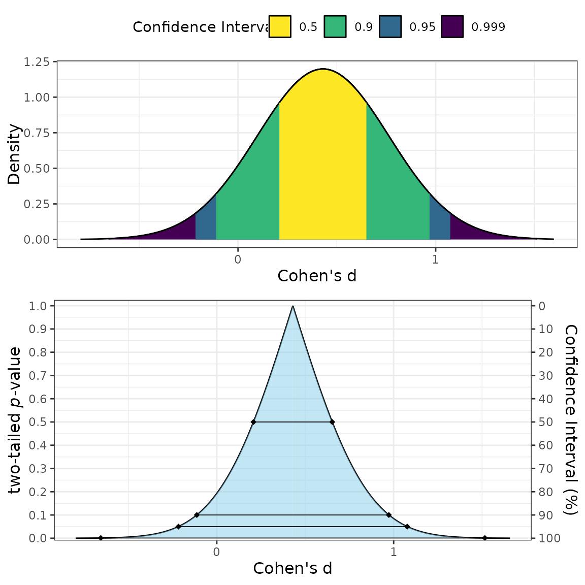
Two types of plots can be produced: consonance
(type = "c"), consonance density
(type = "cd"), or both (the default option;
(type = c("c","cd")))
plot_smd(d = .43,
         df = 58,
         sigma = .33,
         smd_label = "Cohen's d",
         smd_ci = "z"
         )
Comparing SMDs
In some cases, the SMDs between original and replication studies want to be compared. Rather than looking at whether or not a replication attempt is significant, a researcher could compare to see how compatible the SMDs are between the two studies.
For example, say there is original study reports an effect of Cohen’s dz = 0.95 in a paired samples design with 25 subjects. However, a replication doubled the sample size, found a non-significant effect at an SMD of 0.2. Are these two studies compatible? Or, to put it another way, should the replication be considered a failure to replicate?
We can use the compare_smd function to at least measure
how often we would expect a discrepancy between the original and
replication study if the same underlying effect was being measured (also
assuming no publication bias or differences in protocol).
We can see from the results below that, if the null hypothesis were true, we would only expect to see a discrepancy in SMDs between studies, at least this large, ~1% of the time.
compare_smd(smd1 = 0.95,
            n1 = 25,
            smd2 = 0.23,
            n2 = 50,
            paired = TRUE)
#>
#>  Difference in Cohen's dz (paired)
#>
#> data:  Summary Statistics
#> z = 2.5685, p-value = 0.01021
#> alternative hypothesis: true difference in SMDs is not equal to 0
#> sample estimates:
#> difference in SMDs
#>               0.72
Raw Data
The above results are only based on an approximating the differences
between the SMDs. If the raw data is available, then the optimal
solution is the bootstrap the results. This can be accomplished with the
boot_compare_smd function.
For this example, we will simulate some data.
set.seed(4522)
diff_study1 = rnorm(25,.95)
diff_study2 = rnorm(50)
boot_test = boot_compare_smd(x1 = diff_study1,
                             x2 = diff_study2,
                             paired = TRUE)

boot_test
#>
#>  Bootstrapped Differences in SMDs (paired)
#>
#> data:  Bootstrapped
#> z (observed) = 2.887, p-value = 0.006003
#> alternative hypothesis: true difference in SMDs is not equal to 0
#> 95 percent confidence interval:
#>  0.3161207 1.4831351
#> sample estimates:
#> difference in SMDs
#>          0.8058872

# Table of bootstrapped CIs
knitr::kable(boot_test$df_ci, digits = 4)| estimate | lower.ci | upper.ci | |
|---|---|---|---|
| Difference in SMD | 0.8059 | 0.3161 | 1.4831 |
| SMD1 | 0.9418 | 0.5403 | 1.5318 |
| SMD2 | 0.1359 | -0.1420 | 0.4187 |
Visualize
The results of the bootstrapping are stored in the results. So we can even visualize the differences in SMDs.
library(ggplot2)

list_res = boot_test$boot_res
df1 = data.frame(study = c(rep("original",length(list_res$smd1)),
                           rep("replication",length(list_res$smd2))),
                 smd = c(list_res$smd1,list_res$smd2))
ggplot(df1,
            aes(fill = study, color =smd, x = smd))+
 geom_histogram(aes(y=..density..), alpha=0.5,
                position="identity")+
 geom_density(alpha=.2) +
  labs(y = "", x = "SMD (bootstrapped estimates)") +
  theme_classic()
#> `stat_bin()` using `bins = 30`. Pick better value `binwidth`.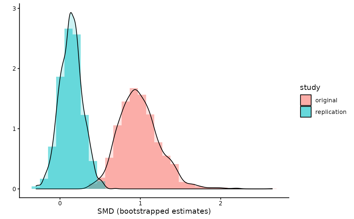
df2 = data.frame(diff = list_res$d_diff)
ggplot(df2,
            aes(x = diff))+
 geom_histogram(aes(y=..density..), alpha=0.5,
                position="identity")+
 geom_density(alpha=.2) +
  labs(y = "", x = "Difference in SMDs (bootstrapped estimates)") +
  theme_classic()
#> `stat_bin()` using `bins = 30`. Pick better value `binwidth`.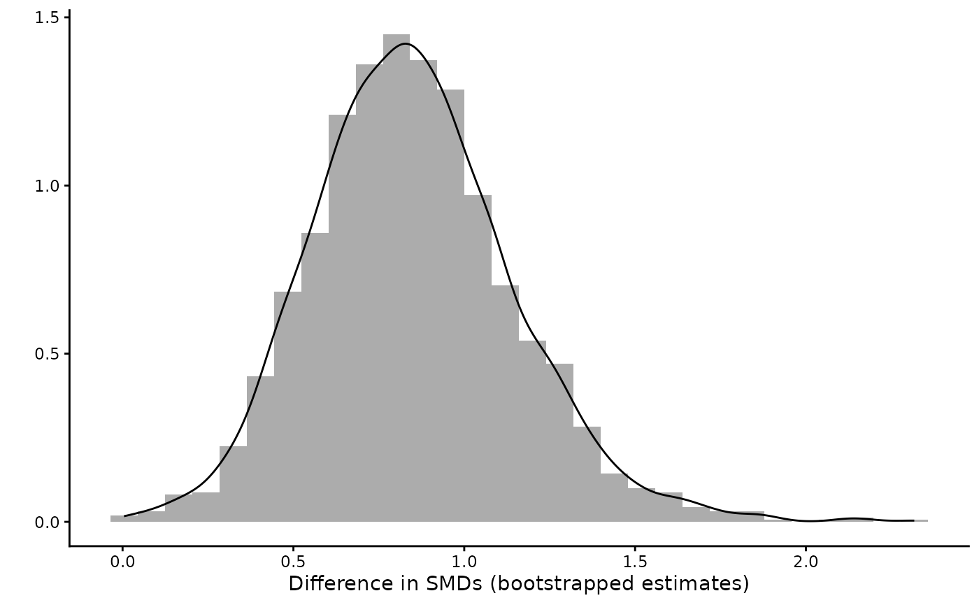
Robust Standardized Mean Differences with Trimming
Motivation
The standard SMD relies on the ordinary mean and standard deviation, which are sensitive to outliers and heavy-tailed distributions. When distributions are non-normal:
- Heavy tails inflate the standard deviation, making the SMD appear smaller than the true distributional separation warrants.
- Outliers can distort the mean difference, pulling the numerator in unpredictable directions.
Algina, Keselman, and Penfield (2005) proposed a robust alternative that uses trimmed means for location and Winsorized variances for scale, with a rescaling constant to maintain comparability with Cohen’s \(\delta\) under normality.
How Trimming Works
Trimmed mean. Given an ordered sample \(x_{(1)} \leq x_{(2)} \leq \cdots \leq
x_{(n)}\) and a trimming proportion \(\gamma\) (the tr argument),
let \(g = \lfloor \gamma \cdot n
\rfloor\) observations be removed from each tail. The trimmed
mean is:
\[ \bar{X}_t = \frac{1}{n - 2g} \sum_{i=g+1}^{n-g} x_{(i)} \]
This reduces the influence of extreme values on the location estimate.
Winsorized variance. Rather than discarding the trimmed observations, Winsorization replaces them with the nearest remaining value. Define the Winsorized sample \(w_i\) as:
\[ w_i = \begin{cases} x_{(g+1)} & \text{if } x_i \leq x_{(g+1)} \\ x_i & \text{if } x_{(g+1)} < x_i < x_{(n-g)} \\ x_{(n-g)} & \text{if } x_i \geq x_{(n-g)} \end{cases} \]
The Winsorized variance is then computed as the ordinary sample variance of the Winsorized values:
\[ S_W^2 = \frac{1}{n-1} \sum_{i=1}^{n} (w_i - \bar{w})^2 \]
This provides a robust scale estimate that down-weights the influence of extreme observations.
Rescaling constant. To ensure the robust SMD equals Cohen’s \(\delta\) under normality, a rescaling constant \(c(\gamma)\) is applied (Algina, Keselman, and Penfield 2005). Let \(a = \Phi^{-1}(1 - \gamma)\) where \(\Phi^{-1}\) is the standard normal quantile function and \(\phi\) is the standard normal density. Then:
\[ c(\gamma) = \sqrt{1 - 2\gamma + 2\gamma a^2 - 2a\,\phi(a)} \]
When \(\gamma = 0\), \(c(0) = 1\) and the formula reduces to the ordinary Cohen’s \(d\). For \(\gamma = 0.2\) (20% trimming), \(c(0.2) \approx 0.642\).
Robust SMD. The robust effect size for two independent samples is then:
\[ d_R = c(\gamma) \cdot \frac{\bar{X}_{t2} - \bar{X}_{t1}}{S_W} \]
where \(S_W\) is based on a pooled,
averaged, or single-group Winsorized standard deviation (depending on
the denom argument), following the same denominator options
as the standard SMD.
Effective sample size. Trimming reduces the effective sample size to \(h = n - 2g\), which replaces \(n\) in all degrees-of-freedom calculations. For example, in the two-sample pooled case with equal trimming, \(df = h_1 + h_2 - 2\).
Usage Examples
All trimming functionality is controlled by the tr
parameter, which defaults to 0 (no trimming):
set.seed(8484)
group1 <- rnorm(40, mean = 100, sd = 15)
group2 <- rnorm(40, mean = 110, sd = 15)

# Standard Cohen's d
smd_calc(x = group1, y = group2, bias_correction = FALSE)
#>
#>  Two Sample Standardized Mean Difference (SMD; Cohen's
#>  d[av]=(x-y)/SD_avg)
#>
#> data:  group1 and group2
#>
#> alternative hypothesis: none
#> 95 percent confidence interval:
#>  -1.2513096 -0.3380927
#> sample estimates:
#> SMD (d[av])
#>  -0.7971844

# Robust version with 20% trimming (Algina et al., 2005)
smd_calc(x = group1, y = group2, bias_correction = FALSE, tr = 0.2)
#>
#>  Two Sample Standardized Mean Difference (SMD; Cohen's
#>  d[av]=(x-y)/SD_avg, 20% trimmed)
#>
#> data:  group1 and group2
#>
#> alternative hypothesis: none
#> 95 percent confidence interval:
#>  -1.2375852 -0.4333599
#> sample estimates:
#> SMD (d[av], 20% trimmed)
#>                -0.839284

# Robust Hedges' g with 10% trimming
smd_calc(x = group1, y = group2, bias_correction = TRUE, tr = 0.1)
#>
#>  Two Sample Standardized Mean Difference (SMD; Hedges's
#>  g[av]=(x-y)/SD_avg, 10% trimmed)
#>
#> data:  group1 and group2
#>
#> alternative hypothesis: none
#> 95 percent confidence interval:
#>  -1.1585132 -0.3166612
#> sample estimates:
#> SMD (g[av], 10% trimmed)
#>               -0.7405285
Bootstrap confidence intervals can also be computed with trimming:
boot_smd_calc(x = group1, y = group2, tr = 0.2, R = 999, boot_ci = "perc")
#>
#>  Two Sample bootstrapped Standardized Mean Difference (SMD; Hedges's
#>  g[av]=(x-y)/SD_avg, 20% trimmed)
#>
#> data:  group1 and group2
#>
#> alternative hypothesis: none
#> 95 percent confidence interval:
#>  -1.3211342 -0.3052718
#> sample estimates:
#> SMD (g[av], 20% trimmed)
#>               -0.8252612
Choosing a Trimming Proportion
-
tr = 0.2(20% trimming) is the most common recommendation in the robust statistics literature and is the default used by Algina et al. -
tr = 0.1offers a compromise between robustness and efficiency. -
tr = 0recovers the standard (non-robust) SMD. - Higher values provide more protection against outliers but lose more information from the tails.
Worked Example with Contaminated Data
To illustrate the benefit of trimming, consider data from a contaminated normal distribution where 10% of observations come from a distribution with much larger variance:
set.seed(7171)
n <- 50

# Clean data from known populations
x_clean <- rnorm(n, mean = 0, sd = 1)
y_clean <- rnorm(n, mean = 0.5, sd = 1)

# Contaminated version: replace 10% with outliers
n_contam <- ceiling(0.1 * n)
x_contam <- c(x_clean[1:(n - n_contam)], rnorm(n_contam, mean = 0, sd = 10))
y_contam <- c(y_clean[1:(n - n_contam)], rnorm(n_contam, mean = 0.5, sd = 10))

# Standard Cohen's d: attenuated by inflated SD
smd_calc(x = x_contam, y = y_contam, bias_correction = FALSE, smd_ci = "z")
#>
#>  Two Sample Standardized Mean Difference (SMD; Cohen's
#>  d[av]=(x-y)/SD_avg)
#>
#> data:  x_contam and y_contam
#>
#> alternative hypothesis: none
#> 95 percent confidence interval:
#>  -0.6777352  0.1182594
#> sample estimates:
#> SMD (d[av])
#>  -0.2797379

# Trimmed version: closer to the true separation
smd_calc(x = x_contam, y = y_contam, bias_correction = FALSE, tr = 0.2, smd_ci = "z")
#>
#>  Two Sample Standardized Mean Difference (SMD; Cohen's
#>  d[av]=(x-y)/SD_avg, 20% trimmed)
#>
#> data:  x_contam and y_contam
#>
#> alternative hypothesis: none
#> 95 percent confidence interval:
#>  -0.4386941  0.2234265
#> sample estimates:
#> SMD (d[av], 20% trimmed)
#>               -0.1076338

# For reference: Cohen's d on the clean data
smd_calc(x = x_clean, y = y_clean, bias_correction = FALSE, smd_ci = "z")
#>
#>  Two Sample Standardized Mean Difference (SMD; Cohen's
#>  d[av]=(x-y)/SD_avg)
#>
#> data:  x_clean and y_clean
#>
#> alternative hypothesis: none
#> 95 percent confidence interval:
#>  -0.5792533  0.2143381
#> sample estimates:
#> SMD (d[av])
#>  -0.1824576
The trimmed SMD is more resistant to the contaminating observations and provides an estimate closer to what we would obtain from the clean data.
Limitations
- The
denom = "rm"option (repeated measures correction) is not currently supported with trimming. - The
smd_ci = "goulet"CI method is not supported with trimming. - The noncentral-t CI with trimming may still have some coverage
issues for very heavy-tailed distributions; the percentile or BCa
bootstrap (via
boot_smd_calc) is recommended in such cases, following Algina et al.’s findings.