Equivalence Testing for F-tests
Aaron R. Caldwell
2026-04-17
the_ftestTOSTER.RmdIntroduction
This vignette demonstrates how to perform equivalence testing for F-tests in ANOVA models using the TOSTER package. While traditional null hypothesis significance testing (NHST) helps determine if effects are different from zero, equivalence testing allows you to determine if effects are small enough to be considered practically equivalent to zero or meaningfully similar.
For an open access tutorial paper explaining how to set equivalence bounds, and how to perform and report equivalence testing for ANOVA models, see Campbell and Lakens (2021). These functions are designed for omnibus tests, and additional testing may be necessary for specific comparisons between groups or conditions1.
The Theory Behind F-test Equivalence Testing
Statistical equivalence testing (or “omnibus non-inferiority testing” as described by Campbell & Lakens, 2021) for F-tests is based on the cumulative distribution function of the non-central F distribution.
These tests answer the question: “Can we reject the hypothesis that the total proportion of variance in outcome Y attributable to X is greater than or equal to the equivalence bound \(\Delta\)?”
The null and alternative hypotheses for equivalence testing with F-tests are:
\[ H_0: \space \eta^2_p \geq \Delta \quad \text{(Effect is meaningfully large)} \]
\[ H_1: \space \eta^2_p < \Delta \quad \text{(Effect is practically equivalent to zero)} \]
Where \(\eta^2_p\) is the partial eta-squared value (proportion of variance explained) and \(\Delta\) is the equivalence bound.
Campbell & Lakens (2021) calculate the p-value for a one-way ANOVA as:
\[ p = p_F(F; J-1, N-J, \frac{N \cdot \Delta}{1-\Delta}) \]
In TOSTER, we use a more generalized approach that can be applied to a variety of designs, including factorial ANOVA. The non-centrality parameter (ncp = \(\lambda\)) is calculated with the equivalence bound and the degrees of freedom:
\[ \lambda_{eq} = \frac{\Delta}{1-\Delta} \cdot(df_1 + df_2 +1) \]
The p-value for the equivalence test (\(p_{eq}\)) can then be calculated from traditional ANOVA results and the distribution function:
\[ p_{eq} = p_F(F; df_1, df_2, \lambda_{eq}) \]
Where:
- \(F\) is the observed F-statistic
- \(df_1\) is the numerator degrees of freedom (effect df)
- \(df_2\) is the denominator degrees of freedom (error df)
- \(\lambda_{eq}\) is the non-centrality parameter calculated from the equivalence bound
Practical Application with TOSTER
Setting Up
First, let’s load the TOSTER package and examine our example dataset:
library(TOSTER)
# Get Data
data("InsectSprays")

# Look at the data structure
head(InsectSprays)
#>   count spray
#> 1    10     A
#> 2     7     A
#> 3    20     A
#> 4    14     A
#> 5    14     A
#> 6    12     A
The InsectSprays dataset contains counts of insects in
agricultural experimental units treated with different insecticides.
Let’s first run a traditional ANOVA to examine the effect of spray type
on insect counts.
Traditional ANOVA
# Build ANOVA
aovtest = aov(count ~ spray,
              data = InsectSprays)

# Display overall results
knitr::kable(broom::tidy(aovtest),
caption = "Traditional ANOVA Test")| term | df | sumsq | meansq | statistic | p.value |
|---|---|---|---|---|---|
| spray | 5 | 2668.833 | 533.76667 | 34.70228 | 0 |
| Residuals | 66 | 1015.167 | 15.38131 | NA | NA |
From the initial analysis, we can see a clear statistically
significant effect of the factor spray (p-value <
0.001). The F-statistic is 34.7 with 5 and 66 degrees of freedom.
Equivalence Testing Using the Raw F-statistic
Now, let’s perform an equivalence test using the
equ_ftest() function. This function requires the
F-statistic, numerator and denominator degrees of freedom, and the
equivalence bound.
For this example, we’ll set the equivalence bound to a partial eta-squared of 0.35. This means we’re testing the null hypothesis that \(\eta^2_p \geq 0.35\) against the alternative that \(\eta^2_p < 0.35\).
equ_ftest(Fstat = 34.70228,
          df1 = 5,
          df2 = 66,
          eqbound = 0.35)
#>
#>  Equivalence Test from F-test
#>
#> data:  Summary Statistics
#> F = 34.702, df1 = 5, df2 = 66, p-value = 1
#> 95 percent confidence interval:
#>  0.5806263 0.7804439
#> sample estimates:
#> [1] 0.724439
Interpreting the Results
Looking at the results:
- The observed partial eta-squared is 0.724, which is quite large
- The equivalence test p-value is 0.999, which is far from significant (p > 0.05)
- The 95% confidence interval for partial eta-squared is [0.592, 0.776]
Based on these results, we would conclude:
- There is a significant effect of “spray” (from the traditional ANOVA)
- The effect is not statistically equivalent to zero (using our equivalence bound of 0.35)
- The observed effect is larger than our equivalence bound of 0.35
In essence, we reject the traditional null hypothesis of “no effect” but fail to reject the null hypothesis of the equivalence test. This could be taken as indication of a meaningfully large effect.
Equivalence Testing Using ANOVA Objects
If you’re doing all your analyses in R, you can use the
equ_anova() function, which accepts objects produced from
stats::aov(), car::Anova(), and
afex::aov_car() (or any ANOVA from afex).
equ_anova(aovtest,
          eqbound = 0.35)
#>        effect df1 df2  F.value       p.null      pes eqbound     p.equ
#> 1 spray         5  66 34.70228 3.182584e-17 0.724439    0.35 0.9999965
The equ_anova() function conveniently provides a data
frame with results for all effects in the model, including the
traditional p-value (p.null), the estimated partial
eta-squared (pes), and the equivalence test p-value
(p.equ).
Minimal Effect Testing
You can also perform minimal effect testing instead of equivalence
testing by setting MET = TRUE. This reverses the
hypotheses:
- Effect is not meaningfully large
\[ H_0: \space \eta^2_p \leq \Delta \] - Effect is meaningfully large
\[ H_1: \space \eta^2_p > \Delta \]
Let’s see how to use this option:
equ_anova(aovtest,
          eqbound = 0.35,
          MET = TRUE)
#>        effect df1 df2  F.value       p.null      pes eqbound        p.equ
#> 1 spray         5  66 34.70228 3.182584e-17 0.724439    0.35 3.502292e-06
In this case, the minimal effect test is significant (p < 0.001), confirming that the effect is meaningfully larger than our bound of 0.35.
Visualizing Partial Eta-Squared
TOSTER provides a function to visualize the uncertainty around
partial eta-squared estimates through consonance plots. The
plot_pes() function requires the F-statistic, numerator
degrees of freedom, and denominator degrees of freedom.
plot_pes(Fstat = 34.70228,
         df1 = 5,
         df2 = 66)
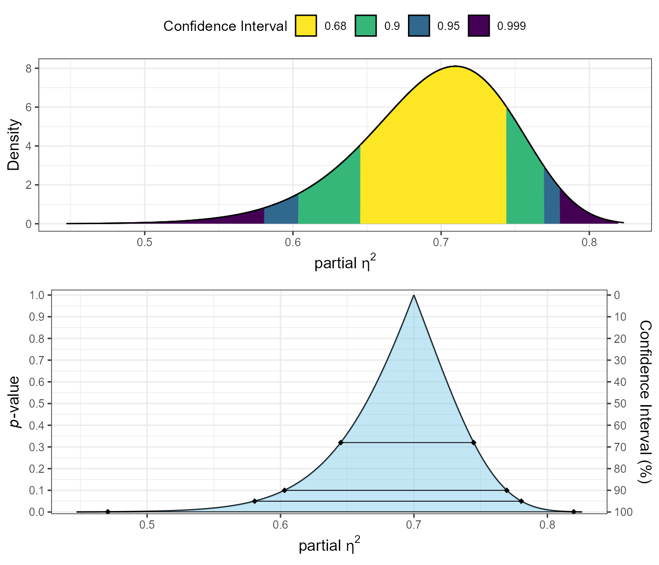
The plots show:
Top plot (Confidence curve): The relationship between p-values and parameter values. The y-axis shows p-values, while the x-axis shows possible values of partial eta-squared. The horizontal lines represent different confidence levels.
Bottom plot (Consonance density): The distribution of plausible values for partial eta-squared. The peak of this distribution represents the most compatible value based on the observed data.
These visualizations help you understand the precision of your effect size estimate and the range of plausible values.
A Second Example: Small Effect
Let’s create a second example with a smaller effect to demonstrate the other possible outcome:
# Simulate data with a small effect
set.seed(123)
groups <- factor(rep(1:3, each = 30))
y <- rnorm(90) + rep(c(0, 0.3, 0.3), each = 30)
small_aov <- aov(y ~ groups)

# Traditional ANOVA
knitr::kable(broom::tidy(small_aov),
caption = "Traditional ANOVA Test (Small Effect)")| term | df | sumsq | meansq | statistic | p.value |
|---|---|---|---|---|---|
| groups | 2 | 4.378103 | 2.189052 | 2.717742 | 0.0716314 |
| Residuals | 87 | 70.075632 | 0.805467 | NA | NA |
# Equivalence test
equ_anova(small_aov, eqbound = 0.15)
#>        effect df1 df2  F.value     p.null      pes eqbound      p.equ
#> 1 groups        2  87 2.717742 0.07163136 0.058803    0.15 0.03619829

# Visualize
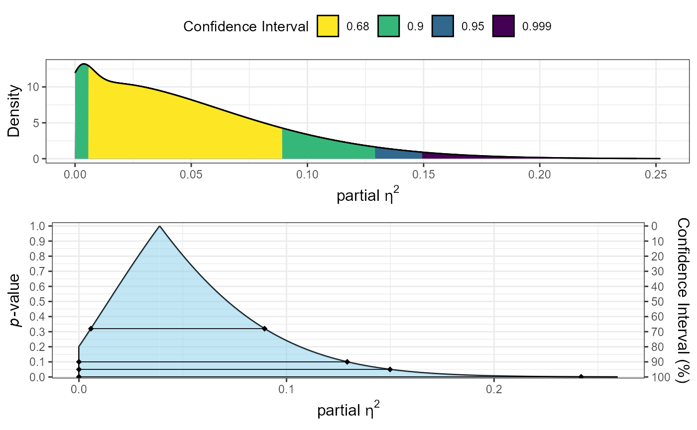
plot_pes(Fstat = 2.36, df1 = 2, df2 = 87)
In this example: 1. The traditional ANOVA shows a marginally significant effect (p = 0.07) 2. The partial eta-squared (0.051) is smaller than our equivalence bound 3. The equivalence test is significant (p < 0.05), indicating the effect is practically equivalent (using our bound of 0.15)
This demonstrates how equivalence testing can help establish that effects are too small to be practically meaningful.
Power Analysis for F-test Equivalence Testing
TOSTER includes a function to calculate power for equivalence
F-tests. The power_eq_f() function allows you to
determine:
- The required sample size for a given power level
- The power for a given amount of degrees of freedom (from which we can infer sample size)
- The detectable equivalence bound for a given power and sample size
Sample Size Calculation
To calculate the sample size needed for 80% power with a specific effect size and equivalence bound:
power_eq_f(df1 = 2,         # Numerator df (groups - 1)
           df2 = NULL,      # Set to NULL to solve for sample size
           eqbound = 0.15,  # Equivalence bound
           power = 0.8)     # Desired power
#> Required df2 = 57.7 (approximately 61 total observations for a one-way ANOVA with 3 groups)
#> Note: This function is primarily validated for one-way ANOVA; use with caution for more complex designs
#>
#>      Power Analysis for F-test Equivalence Testing
#>
#>             df1 = 2
#>             df2 = 57.69827
#>         eqbound = 0.15
#>       sig.level = 0.05
#>           power = 0.8
This tells us we need approximately 60 total participants (yielding df2 = 57) to achieve 80% power for detecting equivalence with a bound of 0.15.
Power Calculation
To calculate the power for a given sample size and equivalence bound:
power_eq_f(df1 = 2,         # Numerator df (groups - 1)
           df2 = 60,        # Error df (N - groups)
           eqbound = 0.15)  # Equivalence bound
#> Power = 0.8189
#> Note: This function is primarily validated for one-way ANOVA; use with caution for more complex designs
#>
#>      Power Analysis for F-test Equivalence Testing
#>
#>             df1 = 2
#>             df2 = 60
#>         eqbound = 0.15
#>       sig.level = 0.05
#>           power = 0.8188512
With 60 error degrees of freedom (about 63 total participants for 3 groups), we would have approximately 80% power to detect equivalence.
Detectable Equivalence Bound
To find the smallest equivalence bound detectable with 80% power given a sample size:
power_eq_f(df1 = 2,         # Numerator df (groups - 1)
           df2 = 60,        # Error df (N - groups)
           power = 0.8)     # Desired power
#> Detectable equivalence bound = 0.1452
#> Note: This function is primarily validated for one-way ANOVA; use with caution for more complex designs
#>
#>      Power Analysis for F-test Equivalence Testing
#>
#>             df1 = 2
#>             df2 = 60
#>         eqbound = 0.1451927
#>       sig.level = 0.05
#>           power = 0.8
With 60 error degrees of freedom, we could detect equivalence at a bound of approximately 0.145 with 80% power.
Choosing Appropriate Equivalence Bounds
Selecting an appropriate equivalence bound is crucial and should be based on:
- Field-specific standards: Some research areas have established conventions
- Smallest effect size of interest: What’s the smallest effect that would be theoretically or practically meaningful?
- Prior research: What effect sizes have been reported in similar studies? Caution is warranted with this approach as previous research is likely to be an overestimate of any “real” effect (i.e., the winner’s curse).
- Resource constraints: Smaller bounds require larger sample sizes
Whatever your choice, it should be adjusted based on your specific research context and questions.
Conclusion
Equivalence testing for F-tests provides a valuable complement to traditional NHST by allowing researchers to establish evidence for the absence of meaningful effects. The TOSTER package offers user-friendly functions for:
- Performing equivalence tests on ANOVA results
(
equ_anova()andequ_ftest()) - Visualizing uncertainty around partial eta-squared estimates
(
plot_pes()) - Conducting power analyses for planning studies
(
power_eq_f())
By incorporating these tools into your analysis workflow, you can make more nuanced inferences about effect sizes and avoid the common pitfall of interpreting non-significant p-values as evidence for the absence of an effect.