An Introduction to t_TOST

Introduction to TOST

TOST (Two One-Sided Tests) is a statistical approach used primarily for equivalence testing. Unlike traditional null hypothesis significance testing which aims to detect differences, equivalence testing aims to statistically support a claim of “no meaningful difference” between groups or conditions. This is particularly useful in bioequivalence studies, non-inferiority trials, or any research where establishing similarity (rather than difference) is the primary goal.

In an effort to make TOSTER more informative and easier to use, I created the functions t_TOST and simple_htest. These functions operate very similarly to base R’s t.test function with a few key enhancements:

t_TOST performs 3 t-tests simultaneously:
- One traditional two-tailed test
- Two one-sided tests to assess equivalence
simple_htest allows you to run equivalence testing or minimal effects testing using either t-tests or Wilcoxon-Mann-Whitney tests, with output in the familiar htest class format (like base R’s statistical test functions).

Both functions have versatile methods where you can supply:

Two vectors of data
A formula interface (e.g., y ~ group)
Various test configurations (two-sample, one-sample, or paired samples)

The functions also provide enhanced summary information and visualizations that make interpreting results more intuitive and user-friendly.

Beyond Equivalence: Minimal Effects Testing

These functions are not limited to equivalence tests. Minimal effects testing (MET) is also supported, which is useful for situations where the hypothesis concerns a minimal effect and the null hypothesis is equivalence. This reverses the typical TOST paradigm and can be valuable in contexts where you want to demonstrate that an effect exceeds some minimal threshold.

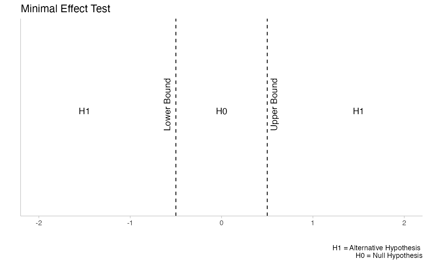
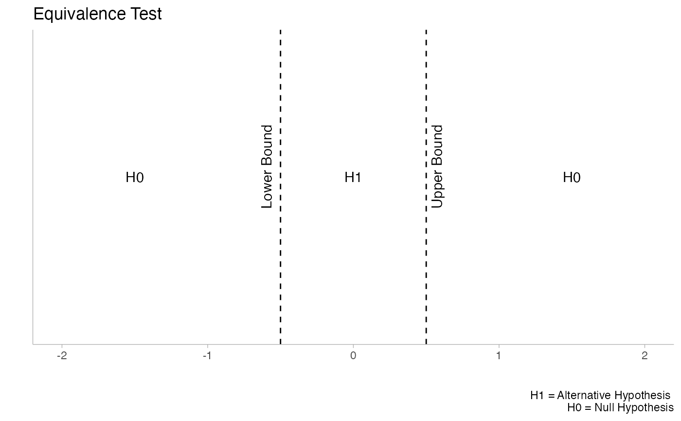
The plots above illustrate the conceptual difference between Minimal Effect Tests (left) and Equivalence Tests (right). Notice how the null (H0) and alternative (H1) hypotheses are reversed between these approaches.

Getting Started with Sample Data

In this vignette, we’ll use the built-in iris and sleep datasets to demonstrate various applications of TOST.

data('sleep')
data('iris')

Let’s take a quick look at the sleep data:

head(sleep)
#>   extra group ID
#> 1   0.7     1  1
#> 2  -1.6     1  2
#> 3  -0.2     1  3
#> 4  -1.2     1  4
#> 5  -0.1     1  5
#> 6   3.4     1  6

The sleep dataset contains observations on the effect of two soporific drugs (group 1 and 2) on 10 patients, with the increase in hours of sleep (extra) as the response variable.

Independent Groups Analysis

Basic Equivalence Testing

For our first example, we’ll test whether the effect of the two drugs in the sleep data is equivalent within bounds of ±0.5 hours. We’ll use both the comprehensive t_TOST function and the simpler simple_htest approach.

Using t_TOST

res1 = t_TOST(formula = extra ~ group,
              data = sleep,
              eqb = .5,  # equivalence bounds of ±0.5 hours
              smd_ci = "t")  # t-distribution for SMD confidence intervals

# Alternative syntax with separate vectors
res1a = t_TOST(x = subset(sleep, group==1)$extra,
               y = subset(sleep, group==2)$extra,
               eqb = .5)

The eqb parameter specifies our equivalence bounds (±0.5 hours of sleep). The smd_ci = "t" argument indicates that we want to use the t-distribution and the standard error of the standardized mean difference (SMD) to create SMD confidence intervals, which is computationally faster for demonstration purposes.

Using simple_htest

We can achieve similar results with the more concise simple_htest function:

# Simple htest approach
res1b = simple_htest(formula = extra ~ group,
                     data = sleep,
                     mu = .5,  # equivalence bound
                     alternative = "e")  # "e" for equivalence

The alternative = "e" specifies an equivalence test, and mu = .5 sets our equivalence bound.

Viewing Results

Let’s examine the output from both approaches:

# Comprehensive t_TOST output
print(res1)
#> 
#> Welch Two Sample t-test
#> 
#> The equivalence test was non-significant, t(17.78) = -1.3, p = 0.89
#> The null hypothesis test was non-significant, t(17.78) = -1.86, p = 0.08
#> NHST: don't reject null significance hypothesis that the effect is equal to zero 
#> TOST: don't reject null equivalence hypothesis
#> 
#> TOST Results 
#>                 t    df p.value
#> t-test     -1.861 17.78   0.079
#> TOST Lower -1.272 17.78   0.890
#> TOST Upper -2.450 17.78   0.012
#> 
#> Effect Sizes 
#>                Estimate     SE               C.I. Conf. Level
#> Raw             -1.5800 0.8491 [-3.0534, -0.1066]         0.9
#> Hedges's g(av)  -0.7965 0.4900  [-1.6467, 0.0537]         0.9
#> Note: SMD confidence intervals are an approximation. See vignette("SMD_calcs").

# Concise htest output
print(res1b)
#> 
#>  Welch Two Sample t-test
#> 
#> data:  extra by group
#> t = -1.2719, df = 17.776, p-value = 0.8901
#> alternative hypothesis: equivalence
#> null values:
#> difference in means difference in means 
#>                -0.5                 0.5 
#> 90 percent confidence interval:
#>  -3.0533815 -0.1066185
#> sample estimates:
#> mean of x mean of y 
#>      0.75      2.33

Notice how t_TOST provides detailed information including both raw and standardized effect sizes, whereas simple_htest gives a more concise summary in the familiar format of base R’s statistical tests.

Visualizing Results

One of the advantages of t_TOST is its built-in visualization capabilities. There are four types of plots available:

1. Simple Dot-and-Whisker Plot

This is the default plot type, showing the point estimate and confidence intervals relative to the equivalence bounds:

plot(res1, type = "simple")

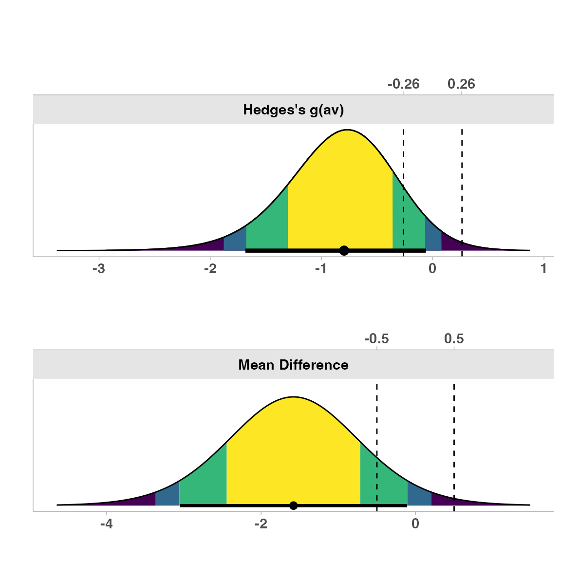
This plot clearly shows where our observed difference (with confidence intervals) falls in relation to our equivalence bounds (dashed vertical lines).

2. Consonance Density Plot

This plot shows the distribution of possible effect sizes, with shading for different confidence levels:

# Shade the 90% and 95% CI areas
plot(res1, type = "cd",
     ci_shades = c(.9, .95))

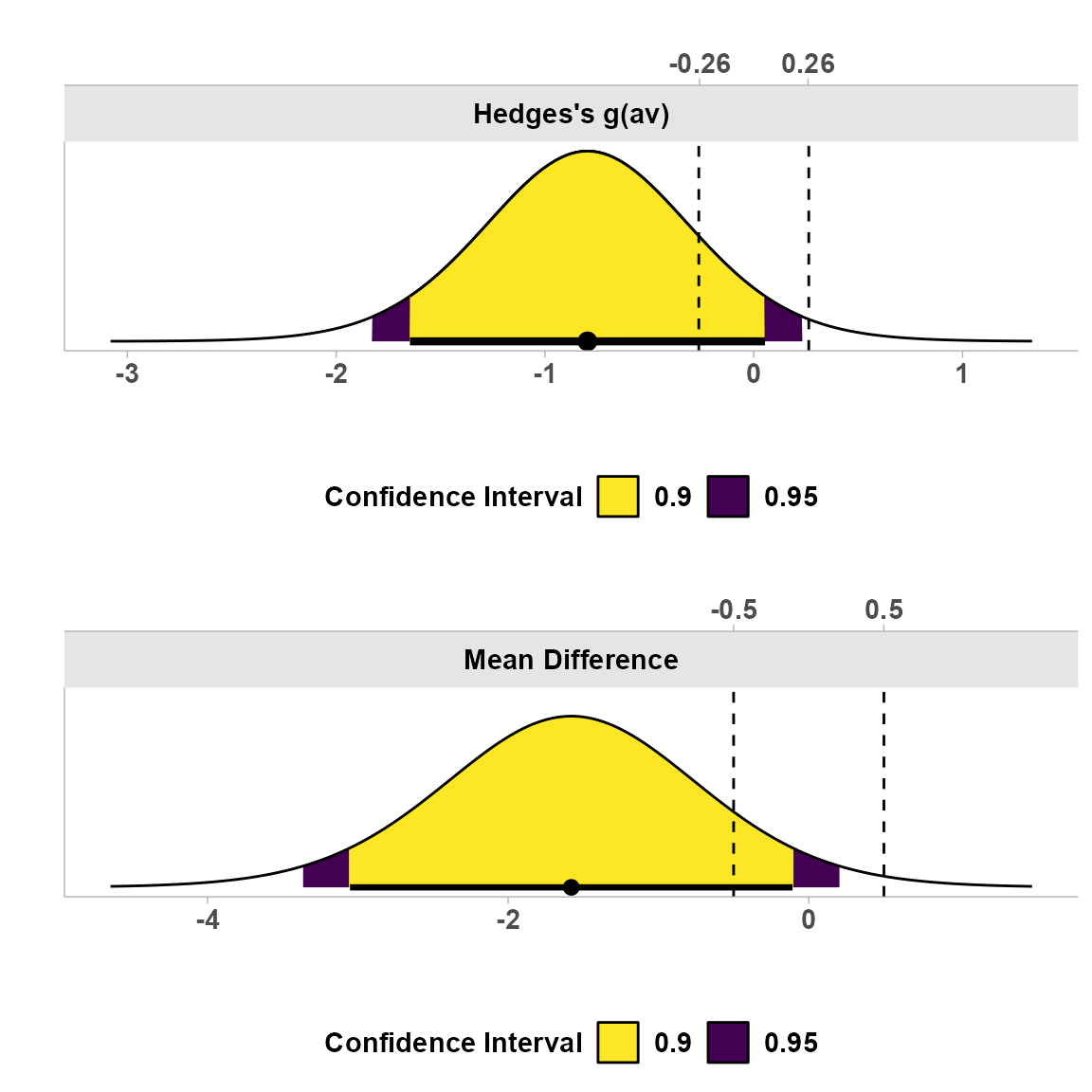
The darker shaded region represents the 90% confidence interval, while the lighter region represents the 95% confidence interval. This visualization helps illustrate the precision of our estimate.

3. Consonance Plot

This plot shows multiple confidence intervals simultaneously:

plot(res1, type = "c",
     ci_lines = c(.9, .95))

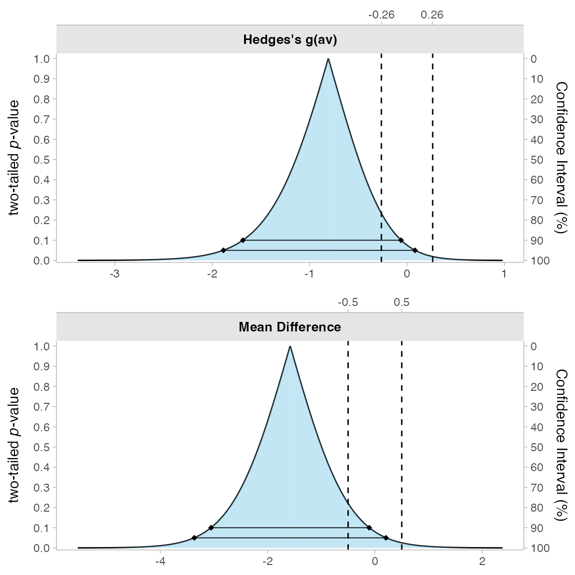
Here, we can see both the 90% and 95% confidence intervals represented as different lines.

4. Null Distribution Plot

This plot visualizes the null distribution:

plot(res1, type = "tnull")
#> SMD cannot be plotted if type = "tnull"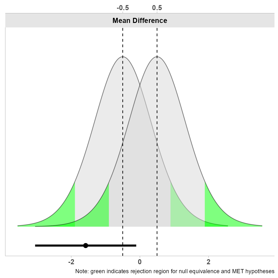

This visualization is particularly useful for understanding the theoretical distribution under the null hypothesis.

Describing Results in Plain Language

Both t_TOST and simple_htest objects can be used with the describe or describe_htest functions to generate plain language interpretations of the results:

describe(res1)
describe_htest(res1b)

Using the Welch Two Sample t-test, a null hypothesis significance test (NHST), and a equivalence test, via two one-sided tests (TOST), were performed with an alpha-level of 0.05. These tested the null hypotheses that true mean difference is equal to 0 (NHST), and true mean difference is more extreme than -0.5 and 0.5 (TOST). Both the equivalence test (p = 0.89), and the NHST (p = 0.079) were not significant (mean difference = -1.58 90% C.I.[-3.05, -0.107]; Hedges’s g(av) = -0.796 90% C.I.[-1.65, 0.054]). Therefore, the results are inconclusive: neither null hypothesis can be rejected.

The Welch Two Sample t-test is not statistically significant (t(17.776) = -1.27, p = 0.89, mean of x = 0.75, mean of y = 2.33, 90% C.I.[-3.05, -0.107]) at a 0.05 alpha-level. The null hypothesis cannot be rejected. At the desired error rate, it cannot be stated that the true difference in means is between -0.5 and 0.5.

These descriptions provide accessible interpretations of the statistical results, making it easier to understand and communicate findings.

Paired Samples Analysis

Many study designs involve paired measurements (e.g., before-after designs or matched samples). Let’s examine how to perform TOST with paired data.

Using the Sleep Data with Paired Analysis

We can use the same sleep data, but now treat the measurements as paired:

res2 = t_TOST(formula = extra ~ group,
              data = sleep,
              paired = TRUE,  # specify paired analysis
              eqb = .5)
res2
#> 
#> Paired t-test
#> 
#> The equivalence test was non-significant, t(9) = -2.8, p = 0.99
#> The null hypothesis test was significant, t(9) = -4.06, p < 0.01
#> NHST: reject null significance hypothesis that the effect is equal to zero 
#> TOST: don't reject null equivalence hypothesis
#> 
#> TOST Results 
#>                 t df p.value
#> t-test     -4.062  9   0.003
#> TOST Lower -2.777  9   0.989
#> TOST Upper -5.348  9 < 0.001
#> 
#> Effect Sizes 
#>               Estimate     SE               C.I. Conf. Level
#> Raw             -1.580 0.3890   [-2.293, -0.867]         0.9
#> Hedges's g(z)   -1.174 0.4412 [-1.8046, -0.4977]         0.9
#> Note: SMD confidence intervals are an approximation. See vignette("SMD_calcs").

res2b = simple_htest(
  formula = extra ~ group,
  data = sleep,
  paired = TRUE,
  mu = .5,
  alternative = "e")
res2b
#> 
#>  Paired t-test
#> 
#> data:  extra by group
#> t = -2.7766, df = 9, p-value = 0.9892
#> alternative hypothesis: equivalence
#> null values:
#> mean difference mean difference 
#>            -0.5             0.5 
#> 90 percent confidence interval:
#>  -2.2930053 -0.8669947
#> sample estimates:
#> mean difference 
#>           -1.58

Setting paired = TRUE changes the analysis to account for within-subject correlations.

Using Separate Vectors for Paired Data

Alternatively, we can provide two separate vectors for paired data, as demonstrated with the iris dataset:

res3 = t_TOST(x = iris$Sepal.Length,
              y = iris$Sepal.Width,
              paired = TRUE,
              eqb = 1)
res3
#> 
#> Paired t-test
#> 
#> The equivalence test was non-significant, t(149) = 22.32, p = 1
#> The null hypothesis test was significant, t(149) = 34.815, p < 0.01
#> NHST: reject null significance hypothesis that the effect is equal to zero 
#> TOST: don't reject null equivalence hypothesis
#> 
#> TOST Results 
#>                t  df p.value
#> t-test     34.82 149 < 0.001
#> TOST Lower 47.31 149 < 0.001
#> TOST Upper 22.32 149       1
#> 
#> Effect Sizes 
#>               Estimate      SE             C.I. Conf. Level
#> Raw              2.786 0.08002 [2.6536, 2.9184]         0.9
#> Hedges's g(z)    2.828 0.18393 [2.5252, 3.1244]         0.9
#> Note: SMD confidence intervals are an approximation. See vignette("SMD_calcs").

res3a = simple_htest(
  x = iris$Sepal.Length,
  y = iris$Sepal.Width,
  paired = TRUE,
  mu = 1,
  alternative = "e"
)
res3a
#> 
#>  Paired t-test
#> 
#> data:  x and y
#> t = 22.319, df = 149, p-value = 1
#> alternative hypothesis: equivalence
#> null values:
#> mean difference mean difference 
#>              -1               1 
#> 90 percent confidence interval:
#>  2.653551 2.918449
#> sample estimates:
#> mean difference 
#>           2.786

Here we’re testing whether the difference between Sepal.Length and Sepal.Width is equivalent within ±1 unit.

Minimal Effect Testing (MET)

As mentioned earlier, sometimes we want to test for a minimal effect rather than equivalence. We can do this by changing the hypothesis argument to “MET”:

res_met = t_TOST(x = iris$Sepal.Length,
              y = iris$Sepal.Width,
              paired = TRUE,
              hypothesis = "MET",  # Change to minimal effect test
              eqb = 1,
              smd_ci = "t")
res_met
#> 
#> Paired t-test
#> 
#> The minimal effect test was significant, t(149) = 47.31, p < 0.01
#> The null hypothesis test was significant, t(149) = 34.815, p < 0.01
#> NHST: reject null significance hypothesis that the effect is equal to zero 
#> TOST: reject null MET hypothesis
#> 
#> TOST Results 
#>                t  df p.value
#> t-test     34.82 149 < 0.001
#> TOST Lower 47.31 149       1
#> TOST Upper 22.32 149 < 0.001
#> 
#> Effect Sizes 
#>               Estimate      SE             C.I. Conf. Level
#> Raw              2.786 0.08002 [2.6536, 2.9184]         0.9
#> Hedges's g(z)    2.828 0.30870 [2.3174, 3.3393]         0.9
#> Note: SMD confidence intervals are an approximation. See vignette("SMD_calcs").

res_metb = simple_htest(x = iris$Sepal.Length,
                       y = iris$Sepal.Width,
                       paired = TRUE,
                       mu = 1,
                       alternative = "minimal.effect")
res_metb
#> 
#>  Paired t-test
#> 
#> data:  x and y
#> t = 22.319, df = 149, p-value < 2.2e-16
#> alternative hypothesis: minimal.effect
#> null values:
#> mean difference mean difference 
#>              -1               1 
#> 90 percent confidence interval:
#>  2.653551 2.918449
#> sample estimates:
#> mean difference 
#>           2.786

For simple_htest, we use alternative = "minimal.effect" to specify MET. The smd_ci = "t" in t_TOST specifies using the t-distribution method for calculating standardized mean difference confidence intervals (this is faster than the default “nct” method).

Interpreting MET Results

describe(res_met)
describe_htest(res_metb)

Using the Paired t-test, a null hypothesis significance test (NHST), and a minimal effect test, via two one-sided tests (TOST), were performed with an alpha-level of 0.05. These tested the null hypotheses that true mean difference is equal to 0 (NHST), and true mean difference is greater than -1 or less than 1 (TOST). The minimal effect test was significant, t(149) = 22.319, p < 0.001 (mean difference = 2.786 90% C.I.[2.654, 2.918]; Hedges’s g(z) = 2.828 90% C.I.[2.317, 3.339]). At the desired error rate, it can be stated that the true mean difference is less than -1 or greater than 1.

The Paired t-test is statistically significant (t(149) = 22.319, p < 0.001, mean difference = 2.786, 90% C.I.[2.654, 2.918]) at a 0.05 alpha-level. The null hypothesis can be rejected. At the desired error rate, it can be stated that the true mean difference is less than -1 or greater than 1.

One Sample t-test

In some cases, we may want to compare a single sample against known bounds. For this, we can use a one-sample test:

res4 = t_TOST(x = iris$Sepal.Length,
              hypothesis = "EQU",
              eqb = c(5.5, 8.5),  # lower and upper bounds
              smd_ci = "t")
res4
#> 
#> One Sample t-test
#> 
#> The equivalence test was significant, t(149) = 5.08, p < 0.01
#> The null hypothesis test was significant, t(149) = 86.425, p < 0.01
#> NHST: reject null significance hypothesis that the effect is equal to zero 
#> TOST: reject null equivalence hypothesis
#> 
#> TOST Results 
#>                  t  df p.value
#> t-test      86.425 149 < 0.001
#> TOST Lower   5.078 149 < 0.001
#> TOST Upper -39.293 149 < 0.001
#> 
#> Effect Sizes 
#>            Estimate      SE             C.I. Conf. Level
#> Raw           5.843 0.06761 [5.7314, 5.9552]         0.9
#> Hedges's g    7.021 0.41350 [6.2039, 7.8381]         0.9
#> Note: SMD confidence intervals are an approximation. See vignette("SMD_calcs").

Here, we’re testing whether the mean of Sepal.Length is equivalent within bounds of 5.5 and 8.5 units. Notice how we specify the bounds as a vector with two distinct values rather than a single value that gets applied symmetrically.

Working with Summary Statistics Only

Researchers often only have access to summary statistics rather than raw data, especially when working with published literature. The tsum_TOST function allows you to perform TOST analyses using just summary statistics:

res_tsum = tsum_TOST(
  m1 = mean(iris$Sepal.Length, na.rm=TRUE),  # sample mean
  sd1 = sd(iris$Sepal.Length, na.rm=TRUE),   # sample standard deviation
  n1 = length(na.omit(iris$Sepal.Length)),  # sample size
  hypothesis = "EQU",
  eqb = c(5.5, 8.5)
)

res_tsum
#> 
#> One-sample t-test
#> 
#> The equivalence test was significant, t(149) = 5.078, p = 5.62e-07
#> The null hypothesis test was significant, t(149) = 86.425, p = 3.33e-129
#> NHST: reject null significance hypothesis that the effect is equal to zero 
#> TOST: reject null equivalence hypothesis
#> 
#> TOST Results 
#>                  t  df p.value
#> t-test      86.425 149 < 0.001
#> TOST Lower   5.078 149 < 0.001
#> TOST Upper -39.293 149 < 0.001
#> 
#> Effect Sizes 
#>            Estimate      SE             C.I. Conf. Level
#> Raw           5.843 0.06761 [5.7314, 5.9552]         0.9
#> Hedges's g    7.021 0.41350  [6.327, 7.6914]         0.9
#> Note: SMD confidence intervals are an approximation. See vignette("SMD_calcs").

Required arguments vary depending on the test type: * n1 & n2: the sample sizes (only n1 needed for one-sample tests) * m1 & m2: the sample means * sd1 & sd2: the sample standard deviations * r12: the correlation between paired samples (only needed if paired = TRUE)

The same visualization and description methods work with tsum_TOST:

plot(res_tsum)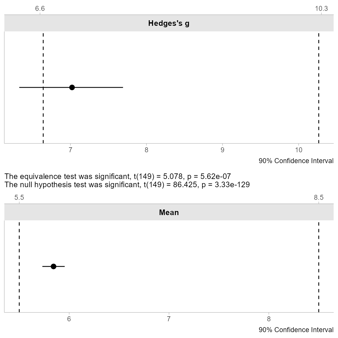

describe(res_tsum)
#> [1] "Using the One-sample t-test, a null hypothesis significance test (NHST), and a equivalence test, via two one-sided tests (TOST), were performed with an alpha-level of 0.05. These tested the null hypotheses that true mean is equal to 0 (NHST), and true mean is more extreme than 5.5 and 8.5 (TOST). The equivalence test was significant, t(149) = 5.078, p < 0.001 (mean = 5.843 90% C.I.[5.731, 5.955]; Hedges's g = 7.021 90% C.I.[6.327, 7.691]). At the desired error rate, it can be stated that the true mean is between 5.5 and 8.5."

Power Analysis for TOST

Planning studies requires determining appropriate sample sizes. The power_t_TOST function allows for power calculations specifically designed for TOST analyses.

This function uses more accurate methods than previous TOSTER functions and matches results from commercial software like PASS. The calculations are based on Owen’s Q-function or direct integration of the bivariate non-central t-distribution¹. Approximate power is implemented via the non-central t-distribution or the ‘shifted’ central t-distribution Diletti, Hauschke, and Steinijans (1992).

The interface mimics base R’s power.t.test function. You specify equivalence bounds and leave one parameter blank (alpha, power, or n) to solve for it:

power_t_TOST(n = NULL,
  delta = 1,          # assumed true difference
  sd = 2.5,           # assumed standard deviation
  eqb = 2.5,          # equivalence bounds
  alpha = .025,       # significance level
  power = .95,        # desired power
  type = "two.sample") # test type
#> 
#>      Two-sample TOST power calculation 
#> 
#>           power = 0.95
#>            beta = 0.05
#>           alpha = 0.025
#>               n = 73.16747
#>           delta = 1
#>              sd = 2.5
#>          bounds = -2.5, 2.5
#> 
#> NOTE: n is number in *each* group

In this example, we’re planning a two-sample equivalence study where: - We assume the true difference is at least 1 unit - The standard deviation is estimated to be 2.5 - We set equivalence bounds to ±2.5 units - We want 95% power with alpha of 0.025

The analysis indicates we need 74 participants per group (148 total) to achieve our desired power.

For more advanced power analysis options, the PowerTOST R package provides additional functionality.

Conclusion

The t_TOST and simple_htest functions in the TOSTER package provide flexible and user-friendly tools for performing equivalence testing and minimal effect testing. With support for various study designs, robust visualization capabilities, and plain language interpretations, these functions make it easier to apply and communicate these important statistical approaches.

Whether you’re analyzing raw data or working with summary statistics, TOSTER provides the tools needed to conduct and interpret these tests appropriately.

References

Diletti, E, D Hauschke, and VW Steinijans. 1992. “Sample Size Determination for Bioequivalence Assessment by Means of Confidence Intervals.” International Journal of Clinical Pharmacology, Therapy, and Toxicology 30 Suppl 1: S51—8.

Labes, Detlew, Helmut Schütz, and Benjamin Lang. 2021. PowerTOST: Power and Sample Size for (Bio)equivalence Studies. https://CRAN.R-project.org/package=PowerTOST.

Phillips, Kem F. 1990. “Power of the Two One-Sided Tests Procedure in Bioequivalence.” Journal of Pharmacokinetics and Biopharmaceutics 18 (2): 137–44. https://doi.org/10.1007/bf01063556.

A new function for TOST with t-tests

Aaron R. Caldwell

2025-03-28