# A tibble: 10 × 12
   subject_id treatment baseline_score  time subject_intercept subject_slope
        <int> <fct>              <dbl> <int>             <dbl>         <dbl>
 1          1 Control             44.4     0              1.90         0.118
 2          1 Control             44.4     1              1.90         0.118
 3          1 Control             44.4     2              1.90         0.118
 4          1 Control             44.4     3              1.90         0.118
 5          2 Control             47.7     0             -2.51        -0.947
 6          2 Control             47.7     1             -2.51        -0.947
 7          2 Control             47.7     2             -2.51        -0.947
 8          2 Control             47.7     3             -2.51        -0.947
 9          3 Control             65.6     0             -1.67        -0.491
10          3 Control             65.6     1             -1.67        -0.491
# ℹ 6 more variables: treatment_effect <dbl>, time_effect <dbl>, error <dbl>,
# outcome <dbl>, time_factor <fct>, subject_factor <fct>7 Module 7: Repeated Measures
7.1 Introduction to Repeated Measures Models
Repeated measures designs occur when multiple measurements of the same response variable are taken from the same experimental unit (subject) over time or under different conditions. This violates the independence assumption of traditional ANOVA because observations from the same subject should be correlated.
7.1.1 Key Characteristics:
- Multiple observations per subject
- Observations within subjects are not independent
- Common in longitudinal studies, clinical trials, and growth studies
- Can involve measurements over time or across different treatment conditions
7.1.2 Two Main Types:
- Repeated Measures in Time: Subjects receive one treatment and are measured multiple times
- Crossover Designs: Subjects receive all treatments in sequence (has special considerations)
7.1.3 The Problem with Traditional ANOVA
Standard ANOVA assumes:
- Independence of observations
- Homogeneity of variance
- Normality of residuals
In repeated measures, the independence assumption is violated because:
- Measurements from the same subject tend to be more similar
- Temporal correlation may exist (closer time points more correlated)
- Subject-specific effects create dependencies
7.1.4 Analytical Approaches for Repeated Measures
7.1.4.1 Multivariate Approach (MANOVA)
MANOVA (Multivariate Analysis of Variance) treats each time point as a separate dependent variable.
Advantages:
- No assumptions about covariance structure
- Can handle missing data patterns
- Provides multivariate tests
Disadvantages:
- Requires more subjects than time points
- Less powerful with many time points
- Cannot easily incorporate continuous time
When to Use:
- Few time points (typically ≤ 4-5)
- Complete data
- Focus on overall multivariate differences
7.1.4.2 Univariate Approach (Repeated Measures ANOVA)
Treats the design as a split-plot in time where:
- Whole plots = subjects (assigned to between-subject treatments)
- Subplots = time points (within-subject factor)
7.1.4.2.1 Sphericity Assumption
Sphericity requires that the variance of differences between all pairs of repeated measures be equal:
\(\text{Var}(Y_i - Y_j) = \text{constant for all } i \neq j\)
Sphericity is equivalent to:
- Compound symmetry when group sizes are equal
- i.e., Homogeneity of covariance matrices across groups
7.1.4.2.2 Sphericity Corrections
When sphericity is violated, F-tests become liberal (increased Type I error).
Mauchly’s Test: Tests the null hypothesis that sphericity holds
- If p > 0.05: Assume sphericity holds
- If p ≤ 0.05: Apply corrections
Common Corrections:
- Greenhouse-Geisser (\(\tilde{\varepsilon}\)): More conservative, works well when \(\tilde{\varepsilon} < 0.75\)
- Huynh-Feldt (\(\hat{\varepsilon}\)): Less conservative, better when \(\hat{\varepsilon} > 0.75\)
- Lower-bound: Most conservative (\(\varepsilon = \frac{1}{k-1}\) where \(k\) = # time points)
7.1.4.2.3 When to Use Repeated Measures ANOVA:
- Sphericity assumption is met (or corrected)
- Balanced design
- Focus on univariate effects
- Traditional approach many researchers expect
7.1.4.3 Mixed Models Approach
Mixed models provide the most flexible framework for repeated measures by explicitly modeling the correlation structure.
7.1.4.3.1 Random Intercept Models
Model: \(Y_{ij} = \mu + \tau_i + b_j + \varepsilon_{ij}\)
Where:
- \(b_j \sim N(0, \sigma_b^2)\) = random subject effect
- \(\varepsilon_{ij} \sim N(0, \sigma^2)\) = residual error
Correlation Structure: Compound symmetry
- Correlation between any two time points within subject = \(\frac{\sigma_b^2}{\sigma_b^2 + \sigma^2}\)
- Same assumption as traditional repeated measures ANOVA
7.1.4.3.2 Mixed Models for Repeated Measures
Allow specification of flexible covariance structures:
Common Structures:
Compound Symmetry (CS)
\(\sigma^2 \times \begin{bmatrix} 1 & \rho & \rho & \rho \\ \rho & 1 & \rho & \rho \\ \rho & \rho & 1 & \rho \\ \rho & \rho & \rho & 1 \end{bmatrix}\)
Autoregressive AR(1)
\(\sigma^2 \times \begin{bmatrix} 1 & \rho & \rho^2 & \rho^3 \\ \rho & 1 & \rho & \rho^2 \\ \rho^2 & \rho & 1 & \rho \\ \rho^3 & \rho^2 & \rho & 1 \end{bmatrix}\)
Unstructured (UN)
- All variances and covariances estimated separately
- Most flexible but requires many parameters
Spatial Power (SP(POW))
- Like AR(1) but for unequally spaced time points
- Correlation = \(\rho^{|t_i - t_j|}\)
7.1.4.3.3 Model Selection
Use Information Criteria to compare covariance structures:
- AIC (Akaike Information Criterion)
- BIC (Bayesian Information Criterion)
- AICC (Corrected AIC - recommended for small samples)
Rule: Smaller values indicate better fit
7.1.4.3.4 Advantages of Mixed Models:
- Handle unbalanced data and missing values
- Flexible covariance modeling
- Can include continuous time
- Provide both population and subject-specific inferences
- Can model non-linear trends
7.1.5 Choosing the Right Approach
| Method | Best When | Limitations |
|---|---|---|
| MANOVA | Few time points, complete data, multivariate focus | Requires n > p, less powerful with many time points |
| RM-ANOVA | Sphericity met, balanced design, traditional analysis | Sphericity assumption, missing data problems |
| Mixed Models | Flexible correlation, missing data, unbalanced design, continuous time | More complex, requires larger samples for complex structures |
7.1.6 Practical Considerations
7.1.6.1 Missing Data
- MANOVA: Requires complete cases or imputation
- RM-ANOVA: Typically uses listwise deletion
- Mixed Models: Use all available data (MAR assumption)
7.1.6.2 Sample Size
- MANOVA: Need \(n >\) number of time points
- RM-ANOVA: Traditional power calculations apply
- Mixed Models: Complex - depends on correlation structure
7.1.6.3 Software Implementation
- R:
afex::aov_4(),lme4::lmer(),nlme::lme(),mmrm::mmrm - SAS:
PROC GLM,PROC MIXED - SPSS: GLM Repeated Measures, MIXED
7.1.7 Summary
Repeated measures designs require special analytical approaches due to within-subject correlation. The choice of method depends on:
- Data structure (balanced vs. unbalanced, missing data)
- Research questions (univariate vs. multivariate)
- Assumptions (sphericity, covariance structure)
- Complexity (simple vs. flexible modeling needs)
Mixed models are increasingly preferred due to their flexibility in handling realistic data situations and explicit modeling of correlation structures, but traditional approaches remain important and widely used in many fields.
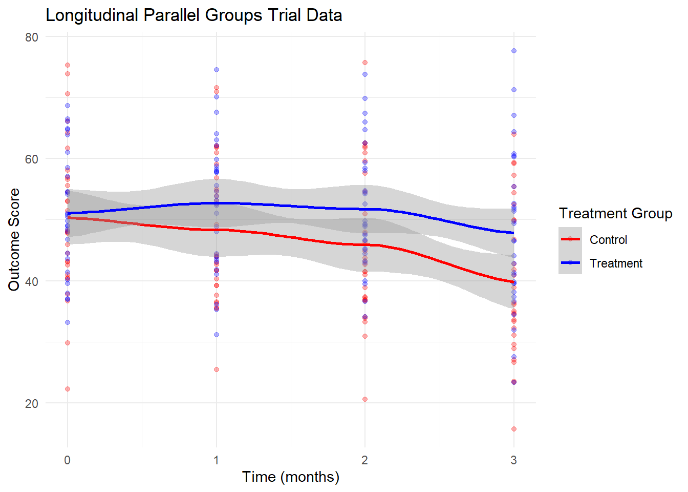
7.2 Using R for Longitudinal Parallel Groups Trials
Longitudinal parallel groups trials are experimental designs where:
- Participants are randomized to different treatment groups at baseline
- Measurements are taken repeatedly over time within each participant
- The primary interest is often in treatment × time interactions
These designs are common in clinical trials, intervention studies, and longitudinal observational research.
7.2.1 Setup and Data Preparation
7.2.2 Method 1: afex::aov_4() - ANOVA Approach
The afex package provides a convenient interface for repeated measures ANOVA using the aov_4() function.
7.2.2.1 Advantages
- Simple syntax similar to base R
aov() - Automatic handling of sphericity corrections
- Built-in post-hoc testing capabilities
- Good for balanced designs
7.2.2.2 Limitations
- Assumes compound symmetry (sphericity)
- Less flexible for handling missing data
- Limited covariance structure options
Univariate Type II Repeated-Measures ANOVA Assuming Sphericity

                      Sum Sq num Df Error SS den Df   F value    Pr(>F)
(Intercept)           564052      1  29157.3     58 1122.0188 < 2.2e-16 ***
treatment               1347      1  29157.3     58    2.6792    0.1071
time_factor             1861      3   1917.4    174   56.3053 < 2.2e-16 ***
treatment:time_factor    421      3   1917.4    174   12.7315  1.46e-07 ***
---
Signif. codes:  0 '***' 0.001 '**' 0.01 '*' 0.05 '.' 0.1 ' ' 1


Mauchly Tests for Sphericity

                      Test statistic p-value
time_factor                  0.86854 0.15659
treatment:time_factor        0.86854 0.15659


Greenhouse-Geisser and Huynh-Feldt Corrections
 for Departure from Sphericity

                       GG eps Pr(>F[GG])
time_factor           0.91165  < 2.2e-16 ***
treatment:time_factor 0.91165  4.462e-07 ***
---
Signif. codes:  0 '***' 0.001 '**' 0.01 '*' 0.05 '.' 0.1 ' ' 1

                         HF eps   Pr(>F[HF])
time_factor           0.9611965 1.352623e-24
treatment:time_factor 0.9611965 2.384340e-07
Anova Table (Type 2 tests)
Response: outcome
num Df den Df MSE F ges Pr(>F)
treatment 1 58 502.71 2.6792 0.041542 0.1071
time_factor 3 174 11.02 56.3053 0.056514 < 2.2e-16 ***
treatment:time_factor 3 174 11.02 12.7315 0.013363 1.46e-07 ***
---
Signif. codes: 0 '***' 0.001 '**' 0.01 '*' 0.05 '.' 0.1 ' ' 1Anova Table (Type 2 tests)
Response: outcome
num Df den Df MSE F ges Pr(>F)
treatment 1.0000 58.00 502.71 2.6792 0.041542 0.1071
time_factor 2.8836 167.25 11.46 56.3053 0.056514 < 2.2e-16 ***
treatment:time_factor 2.8836 167.25 11.46 12.7315 0.013363 2.384e-07 ***
---
Signif. codes: 0 '***' 0.001 '**' 0.01 '*' 0.05 '.' 0.1 ' ' 1Anova Table (Type 2 tests)
Response: outcome
num Df den Df MSE F ges Pr(>F)
treatment 1.0000 58.00 502.71 2.6792 0.041542 0.1071
time_factor 2.7349 158.63 12.09 56.3053 0.056514 < 2.2e-16 ***
treatment:time_factor 2.7349 158.63 12.09 12.7315 0.013363 4.462e-07 ***
---
Signif. codes: 0 '***' 0.001 '**' 0.01 '*' 0.05 '.' 0.1 ' ' 1
Type II Repeated Measures MANOVA Tests: Pillai test statistic
                      Df test stat approx F num Df den Df    Pr(>F)
(Intercept)            1   0.95085  1122.02      1     58 < 2.2e-16 ***
treatment              1   0.04415     2.68      1     58    0.1071
time_factor            1   0.67260    38.35      3     56 1.323e-13 ***
treatment:time_factor  1   0.35973    10.49      3     56 1.415e-05 ***
---
Signif. codes:  0 '***' 0.001 '**' 0.01 '*' 0.05 '.' 0.1 ' ' 1
time_factor = X0:
contrast estimate SE df t.ratio p.value
Control - Treatment -0.729 2.91 58 -0.251 0.8028
time_factor = X1:
contrast estimate SE df t.ratio p.value
Control - Treatment -4.384 2.84 58 -1.546 0.1275
time_factor = X2:
contrast estimate SE df t.ratio p.value
Control - Treatment -5.835 2.92 58 -2.001 0.0501
time_factor = X3:
contrast estimate SE df t.ratio p.value
Control - Treatment -8.003 3.27 58 -2.445 0.01757.2.3 Method 2: lme4::lmer() - Linear Mixed-Effects Models
The lme4 package is the most popular R package for fitting linear mixed-effects models.
7.2.3.1 Advantages
- Very flexible random effects specification
- Efficient computation using sparse matrix methods
- Extensive ecosystem of supporting packages
- Handles unbalanced data well
7.2.3.2 Limitations
- Limited covariance structure options (only random effects)
- No built-in degrees of freedom calculation
- Requires additional packages for p-values
Linear mixed model fit by REML. t-tests use Satterthwaite's method [
lmerModLmerTest]
Formula: outcome ~ treatment * time_factor + (1 | subject_factor)
   Data: data_long

REML criterion at convergence: 1463.9

Scaled residuals:
     Min       1Q   Median       3Q      Max
-2.48484 -0.48718 -0.02863  0.53306  2.36070

Random effects:
 Groups         Name        Variance Std.Dev.
 subject_factor (Intercept) 122.92   11.09
 Residual                    11.02    3.32
Number of obs: 240, groups:  subject_factor, 60

Fixed effects:
                                Estimate Std. Error       df t value Pr(>|t|)
(Intercept)                      50.3456     2.1130  65.7840  23.827  < 2e-16
treatmentTreatment                0.7294     2.9882  65.7840   0.244  0.80792
time_factor1                     -1.9932     0.8571 174.0000  -2.326  0.02120
time_factor2                     -4.4277     0.8571 174.0000  -5.166 6.50e-07
time_factor3                    -10.5212     0.8571 174.0000 -12.275  < 2e-16
treatmentTreatment:time_factor1   3.6549     1.2121 174.0000   3.015  0.00295
treatmentTreatment:time_factor2   5.1052     1.2121 174.0000   4.212 4.06e-05
treatmentTreatment:time_factor3   7.2738     1.2121 174.0000   6.001 1.11e-08

(Intercept)                     ***
treatmentTreatment
time_factor1                    *
time_factor2                    ***
time_factor3                    ***
treatmentTreatment:time_factor1 **
treatmentTreatment:time_factor2 ***
treatmentTreatment:time_factor3 ***
---
Signif. codes:  0 '***' 0.001 '**' 0.01 '*' 0.05 '.' 0.1 ' ' 1

Correlation of Fixed Effects:
            (Intr) trtmnT tm_fc1 tm_fc2 tm_fc3 trT:_1 trT:_2
trtmntTrtmn -0.707
time_factr1 -0.203  0.143
time_factr2 -0.203  0.143  0.500
time_factr3 -0.203  0.143  0.500  0.500
trtmntTr:_1  0.143 -0.203 -0.707 -0.354 -0.354
trtmntTr:_2  0.143 -0.203 -0.354 -0.707 -0.354  0.500
trtmntTr:_3  0.143 -0.203 -0.354 -0.354 -0.707  0.500  0.500
Linear mixed model fit by REML. t-tests use Satterthwaite's method [
lmerModLmerTest]
Formula: outcome ~ treatment * time_factor + (1 | subject_factor)
Data: data_long
REML criterion at convergence: 1463.9
Scaled residuals:
Min 1Q Median 3Q Max
-2.48484 -0.48718 -0.02863 0.53306 2.36070
Random effects:
Groups Name Variance Std.Dev.
subject_factor (Intercept) 122.92 11.09
Residual 11.02 3.32
Number of obs: 240, groups: subject_factor, 60
Fixed effects:
Estimate Std. Error df t value Pr(>|t|)
(Intercept) 50.3456 2.1130 65.7840 23.827 < 2e-16
treatmentTreatment 0.7294 2.9882 65.7840 0.244 0.80792
time_factor1 -1.9932 0.8571 174.0000 -2.326 0.02120
time_factor2 -4.4277 0.8571 174.0000 -5.166 6.50e-07
time_factor3 -10.5212 0.8571 174.0000 -12.275 < 2e-16
treatmentTreatment:time_factor1 3.6549 1.2121 174.0000 3.015 0.00295
treatmentTreatment:time_factor2 5.1052 1.2121 174.0000 4.212 4.06e-05
treatmentTreatment:time_factor3 7.2738 1.2121 174.0000 6.001 1.11e-08
(Intercept) ***
treatmentTreatment
time_factor1 *
time_factor2 ***
time_factor3 ***
treatmentTreatment:time_factor1 **
treatmentTreatment:time_factor2 ***
treatmentTreatment:time_factor3 ***
---
Signif. codes: 0 '***' 0.001 '**' 0.01 '*' 0.05 '.' 0.1 ' ' 1
Correlation of Fixed Effects:
(Intr) trtmnT tm_fc1 tm_fc2 tm_fc3 trT:_1 trT:_2
trtmntTrtmn -0.707
time_factr1 -0.203 0.143
time_factr2 -0.203 0.143 0.500
time_factr3 -0.203 0.143 0.500 0.500
trtmntTr:_1 0.143 -0.203 -0.707 -0.354 -0.354
trtmntTr:_2 0.143 -0.203 -0.354 -0.707 -0.354 0.500
trtmntTr:_3 0.143 -0.203 -0.354 -0.354 -0.707 0.500 0.500Analysis of Deviance Table (Type II Wald chisquare tests)
Response: outcome
Chisq Df Pr(>Chisq)
treatment 2.6792 1 0.1017
time_factor 168.9160 3 < 2.2e-16 ***
treatment:time_factor 38.1946 3 2.571e-08 ***
---
Signif. codes: 0 '***' 0.001 '**' 0.01 '*' 0.05 '.' 0.1 ' ' 1time_factor = 0:
contrast estimate SE df t.ratio p.value
Control - Treatment -0.729 2.99 65.8 -0.244 0.8079
time_factor = 1:
contrast estimate SE df t.ratio p.value
Control - Treatment -4.384 2.99 65.8 -1.467 0.1471
time_factor = 2:
contrast estimate SE df t.ratio p.value
Control - Treatment -5.835 2.99 65.8 -1.953 0.0551
time_factor = 3:
contrast estimate SE df t.ratio p.value
Control - Treatment -8.003 2.99 65.8 -2.678 0.0093
Degrees-of-freedom method: kenward-roger 7.2.4 Method 3: nlme::lme() - Linear Mixed-Effects with Flexible Covariance
The nlme package provides more flexibility in specifying covariance structures.
7.2.4.1 Advantages
- Multiple covariance structure options
- Built-in p-values and confidence intervals
- Flexible correlation and variance structures
- Good for modeling heteroscedasticity
7.2.4.2 Limitations
- Older computational methods (can be slower)
- More complex syntax for some specifications
- Less extensive supporting ecosystem
Linear mixed-effects model fit by REML
  Data: data_long
       AIC     BIC    logLik
  1485.896 1523.81 -731.9481

Random effects:
 Formula: ~1 | subject_factor
        (Intercept) Residual
StdDev:    11.08707 3.319528

Correlation Structure: Compound symmetry
 Formula: ~time_factor | subject_factor
 Parameter estimate(s):
Rho
  0
Fixed effects:  outcome ~ treatment * time_factor
                                    Value Std.Error  DF    t-value p-value
(Intercept)                      50.34562 2.1129942 174  23.826671  0.0000
treatmentTreatment                0.72941 2.9882251  58   0.244096  0.8080
time_factor1                     -1.99323 0.8570984 174  -2.325561  0.0212
time_factor2                     -4.42771 0.8570984 174  -5.165934  0.0000
time_factor3                    -10.52121 0.8570984 174 -12.275382  0.0000
treatmentTreatment:time_factor1   3.65486 1.2121202 174   3.015261  0.0030
treatmentTreatment:time_factor2   5.10524 1.2121202 174   4.211824  0.0000
treatmentTreatment:time_factor3   7.27384 1.2121202 174   6.000923  0.0000
 Correlation:
                                (Intr) trtmnT tm_fc1 tm_fc2 tm_fc3 trT:_1
treatmentTreatment              -0.707
time_factor1                    -0.203  0.143
time_factor2                    -0.203  0.143  0.500
time_factor3                    -0.203  0.143  0.500  0.500
treatmentTreatment:time_factor1  0.143 -0.203 -0.707 -0.354 -0.354
treatmentTreatment:time_factor2  0.143 -0.203 -0.354 -0.707 -0.354  0.500
treatmentTreatment:time_factor3  0.143 -0.203 -0.354 -0.354 -0.707  0.500
                                trT:_2
treatmentTreatment
time_factor1
time_factor2
time_factor3
treatmentTreatment:time_factor1
treatmentTreatment:time_factor2
treatmentTreatment:time_factor3  0.500

Standardized Within-Group Residuals:
        Min          Q1         Med          Q3         Max
-2.48483509 -0.48717550 -0.02862546  0.53305570  2.36069512

Number of Observations: 240
Number of Groups: 60
Analysis of Deviance Table (Type II tests)
Response: outcome
Chisq Df Pr(>Chisq)
treatment 2.6792 1 0.1017
time_factor 168.9160 3 < 2.2e-16 ***
treatment:time_factor 38.1946 3 2.571e-08 ***
---
Signif. codes: 0 '***' 0.001 '**' 0.01 '*' 0.05 '.' 0.1 ' ' 1time_factor = 0:
contrast estimate SE df t.ratio p.value
Control - Treatment -0.729 2.99 58 -0.244 0.8080
time_factor = 1:
contrast estimate SE df t.ratio p.value
Control - Treatment -4.384 2.99 58 -1.467 0.1477
time_factor = 2:
contrast estimate SE df t.ratio p.value
Control - Treatment -5.835 2.99 58 -1.953 0.0557
time_factor = 3:
contrast estimate SE df t.ratio p.value
Control - Treatment -8.003 2.99 58 -2.678 0.0096
Degrees-of-freedom method: containment 7.2.5 Method 4: mmrm::mmrm() - Mixed Models for Repeated Measures
The mmrm package is specifically designed for repeated measures analysis, particularly in clinical trials.
7.2.5.1 Advantages
- Designed specifically for repeated measures
- Multiple covariance structures optimized for repeated measures
- Handles missing data well (MAR assumption)
- Fast computation
- Clinical trial-focused features
7.2.5.2 Limitations
- Newer package with smaller ecosystem
- Focused specifically on repeated measures (less general)
- Fewer supporting packages
mmrm fit

Formula:
outcome ~ treatment * time_factor + ar1(time_factor | subject_factor)
Data:        data_long (used 240 observations from 60 subjects with maximum 4
timepoints)
Covariance:  auto-regressive order one (2 variance parameters)
Method:      Kenward-Roger
Vcov Method: Kenward-Roger
Inference:   REML

Model selection criteria:
     AIC      BIC   logLik deviance
  1484.9   1489.1   -740.4   1480.9

Coefficients:
                                Estimate Std. Error       df t value Pr(>|t|)
(Intercept)                      50.3456     2.1561  69.2600  23.350  < 2e-16
treatmentTreatment                0.7294     3.0492  69.2600   0.239 0.811647
time_factor1                     -1.9932     0.7939 172.8100  -2.511 0.012971
time_factor2                     -4.4277     1.1043 183.9700  -4.009 8.84e-05
time_factor3                    -10.5212     1.3305 194.5900  -7.907 1.92e-13
treatmentTreatment:time_factor1   3.6549     1.1228 172.8100   3.255 0.001363
treatmentTreatment:time_factor2   5.1052     1.5618 183.9700   3.269 0.001289
treatmentTreatment:time_factor3   7.2738     1.8817 194.5900   3.866 0.000151

(Intercept)                     ***
treatmentTreatment
time_factor1                    *
time_factor2                    ***
time_factor3                    ***
treatmentTreatment:time_factor1 **
treatmentTreatment:time_factor2 **
treatmentTreatment:time_factor3 ***
---
Signif. codes:  0 '***' 0.001 '**' 0.01 '*' 0.05 '.' 0.1 ' ' 1

Covariance estimate:
         0        1        2        3
0 141.5101 131.9169 122.9740 114.6373
1 131.9169 141.5101 131.9169 122.9740
2 122.9740 131.9169 141.5101 131.9169
3 114.6373 122.9740 131.9169 141.5101
Analysis of Fixed Effect Table (Type II F tests)
Df Res.Df F Pr(>F)
treatment 1 58.844 2.6300 0.110208
time_factor 3 172.975 30.4041 7.745e-16 ***
treatment:time_factor 3 172.975 5.6259 0.001056 **
---
Signif. codes: 0 '***' 0.001 '**' 0.01 '*' 0.05 '.' 0.1 ' ' 1 0 1 2 3
0 141.5101 131.9169 122.9740 114.6373
1 131.9169 141.5101 131.9169 122.9740
2 122.9740 131.9169 141.5101 131.9169
3 114.6373 122.9740 131.9169 141.5101time_factor = 0:
contrast estimate SE df t.ratio p.value
Control - Treatment -0.729 3.05 69.3 -0.239 0.8116
time_factor = 1:
contrast estimate SE df t.ratio p.value
Control - Treatment -4.384 3.05 69.3 -1.438 0.1550
time_factor = 2:
contrast estimate SE df t.ratio p.value
Control - Treatment -5.835 3.05 69.3 -1.913 0.0598
time_factor = 3:
contrast estimate SE df t.ratio p.value
Control - Treatment -8.003 3.05 69.3 -2.625 0.01077.2.6 Model Comparison
7.2.6.1 Comparing Model Fits
# A tibble: 4 × 3
  Method             AIC   BIC
  <chr>            <dbl> <dbl>
1 afex::aov_4        NA    NA
2 lme4::lmer       1484. 1519.
3 nlme::lme (CS)   1486. 1524.
4 mmrm::mmrm (AR1) 1485. 1489.
7.2.7 Choosing the Right Method
7.2.7.1 Decision Framework
| Factor | Best Choice | Rationale |
|---|---|---|
| Balanced design, simple analysis | afex::aov_4() | Simple syntax, automatic corrections |
| Flexible random effects needed | lme4::lmer() | Most flexible random effects specification |
| Specific covariance structure important | nlme::lme() | Widest variety of covariance structures |
| Clinical trial context | mmrm::mmrm() | Purpose-built for repeated measures |
| Missing data handling | nlme::lme() or mmrm::mmrm() | Sophisticated missing data assumptions |
| Computational efficiency | lme4::lmer() or mmrm::mmrm() | Optimized computational algorithms |
| Ecosystem support | lme4::lmer() | Largest number of supporting packages |
7.2.7.2 Practical Recommendations
For beginners or simple analyses: - Start with afex::aov_4() for balanced designs - Use lme4::lmer() with lmerTest for basic mixed models
For complex covariance modeling: - Use nlme::lme() when you need specific correlation structures - Consider mmrm::mmrm() for clinical trial analyses
For production analyses: - lme4::lmer() for general mixed modeling - mmrm::mmrm() for repeated measures in regulated environments
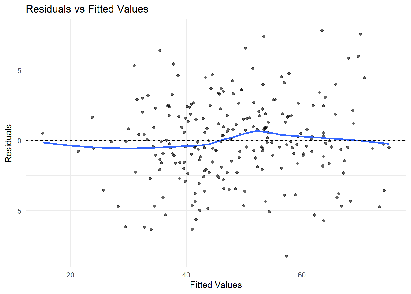
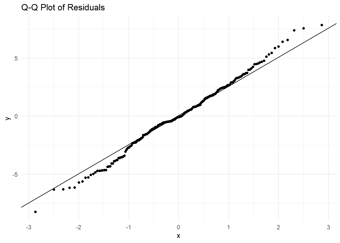
7.2.8 Diagnostic Plots and Model Checking
7.2.9 Summary and Key Takeaways
7.2.9.1 Method Comparison Summary
- afex::aov_4(): Best for simple, balanced repeated measures ANOVA
- lme4::lmer(): Most versatile and widely used mixed-effects modeling
- nlme::lme(): Superior for complex covariance structure specification
- mmrm::mmrm(): Specialized for clinical trial repeated measures
7.2.9.2 Statistical Considerations
- Missing Data: All methods except
afexhandle missing data well under MAR assumptions - Covariance Structure: Choice can significantly impact results and interpretation
- Degrees of Freedom: Different methods use different approximations
- Model Selection: Use information criteria (AIC/BIC) and biological plausibility
7.2.9.3 Best Practices
- Always visualize your data before modeling
- Consider the covariance structure carefully
- Check model assumptions with diagnostic plots
- Report the method and software versions used
- Consider sensitivity analyses with different approaches