2 Module 2: Data, Models, and Association

knitr::opts_chunk$set(echo = FALSE, tidy = TRUE, 
                      cache = FALSE, 
                      message = FALSE, WARNING = FALSE)
# Very standard packages
library(graphics)
library(ggplot2)
library(tidyverse)
library(knitr)
library(readr)
library(MASS)
library(plotly)
library(flextable)

# Not so standard
library(gridExtra) # for grid.arrange(), grids of plots in ggplot without facet_grid
library(ggpubr) #for stat_cor function which adds correlation coefficient to ggplot
library(energy) # distance correlation function and t-test in here
library(scatterplot3d) # for easy/boring scatterplots that work in PDF knit

# Good for running
library(ggstatsplot)
# Globally changing the default ggplot theme.


# I do not want default theme.
old.theme <- theme_get()
theme_set(theme_bw())

2.1 Data

2.1.1 Variables and Observations

Let’s talk about what we mean by data, in this course.

Data is composed of variables and observations.

Example: We have a patient. We measure their blood pressure. It is observed to be 133/86.

Variable: Blood pressure

Observation: 133/86

Or we could reformulate this

Variables: Systolic blood pressure and diastolic blood pressure.

Observation(s): 133 and 86

2.1.2 Heart data introduction

heart <- read_csv(here::here("datasets", "Heart.csv"))

as_flextable(head(heart))

age	sex	chestPain	restSysBP	cholesterol	fastBldSgr	restECG	maxHR	exAng	slope	majorVessels	disease
numeric	character	character	numeric	numeric	numeric	numeric	numeric	numeric	numeric	numeric	character
63	Male	typical	145	233	1	2	150	0	3	0	No
67	Male	asymptomatic	160	286	0	2	108	1	2	3	Yes
67	Male	asymptomatic	120	229	0	2	129	1	2	2	Yes
37	Male	nonanginal	130	250	0	0	187	0	3	0	No
41	Female	nontypical	130	204	0	2	172	0	1	0	No
56	Male	nontypical	120	236	0	0	178	0	1	0	No
n: 6

2.1.3 Heart Disease Data Dictionary

A data dictionary explains what the “names” of variables in a dataset mean. For the heart data:

age: The patient’s age in years
sex: The patient’s sex, Male or Female.
chestPain: The chest pain experienced
- typical: typical angina
- nontypical’: abnormal angina
- nonaginal: non-anginal pain
- asymptomatic: no pain
restSysBP: systolic blood pressure upon admission to hospital in mm Hg
cholesterol: The patient’s cholesterol measurement in mg/dl
fastBldSgr: indicator for whether the paitient’s fasting blood sugar was greater than 120 mg/dl: 1 if yes, 0 if no.
restECG: Resting electrocardiographic measurement
- 0: normal
- 1: having ST-T wave abnormality
- 2 showing probable or definite left ventricular hypertrophy by Estes’ criteria
maxHR: The patient’s maximum heart rate achieved during controlled exercise
exAng: Exercise induced angina: 1 if yes, 0 if no
slope: the slope of the peak exercise ST segment
- 1 if slope is positive
- 2 if slope is approximately 0
- 3 if slope is negative
majorVessels: The number of major vessels (0-3) colored in fluoroscopy.
disease: Indicates whether a patient had heart disease: Yes if yes, no if no.

2.2 Mathematical Models

2.2.1 input and output

The general form of a model is deceptively simple:

\[input \to output.\]

We have some information, the input, we use some process, \(\to\), in order to get some information, the output.

Model: put a quarter in the gumball machine, turn the knob, and a gumball comes out.

Figure 2.1: We have quarter as input to the process, gumball machine, which allows to yield a

2.2.2 Mathematical models

We are doing math here. We will represent our input as \(x\), and our output as \(y\). We put our input \(x\) into some function \(g()\).

\[y = g(x)\]

\(x\) is the input
\(g\) is the \(\to\)
\(y\) is the output

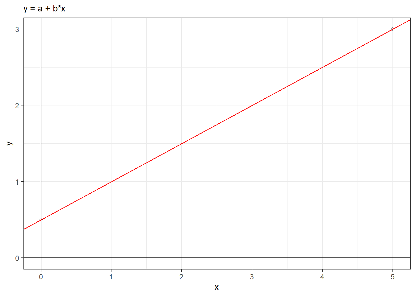
\[ y = a + b \cdot x \]

2.2.3 Heart Model

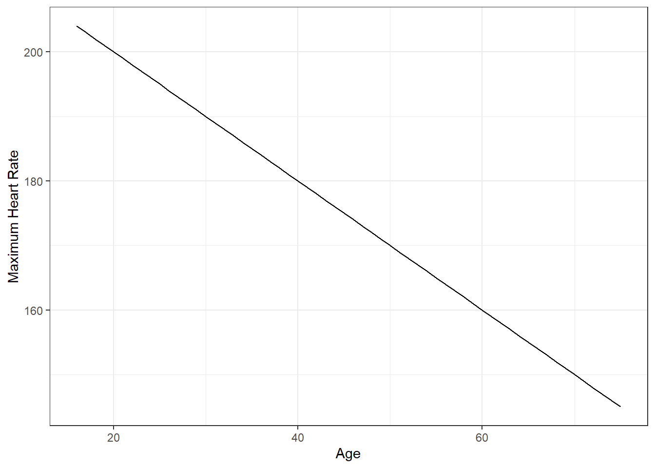
The Mayo Clinic says “You can calculate your maximum heart rate by subtracting your age from 220”.

\(maxHR = 220 - age\)
\(y = 220 - x\)
- y is maxHR
- x is age

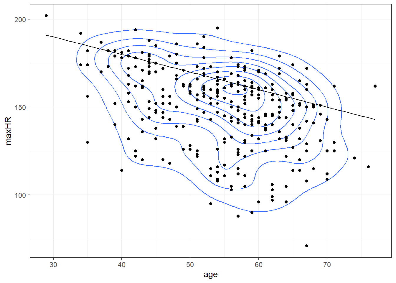
2.2.3.1 What about with the real data?

2.3 Statistical models and Error

\[y = g(x) + \epsilon\]

y = response
x = predictor
g(x) = function
\(\epsilon\) = error or variability in the model

2.3.1 Heart example

The Mayo Clinic also specifies “You may have a higher or lower maximum heart rate, sometimes by as much as 15 to 20 beats per minute”.

\[MaxHR = 220 - age \pm 20\]

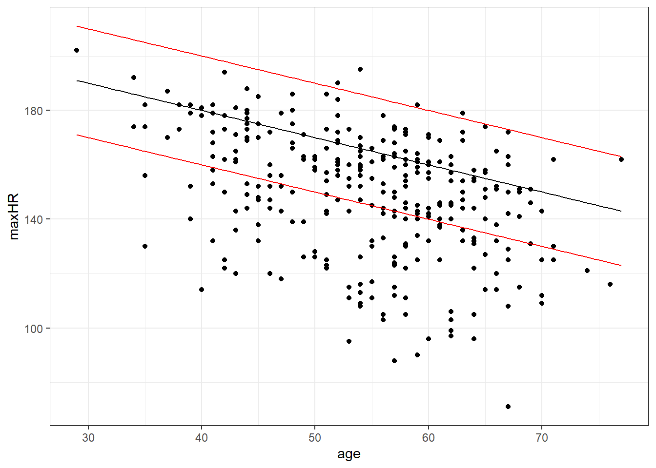
What’s going on here?

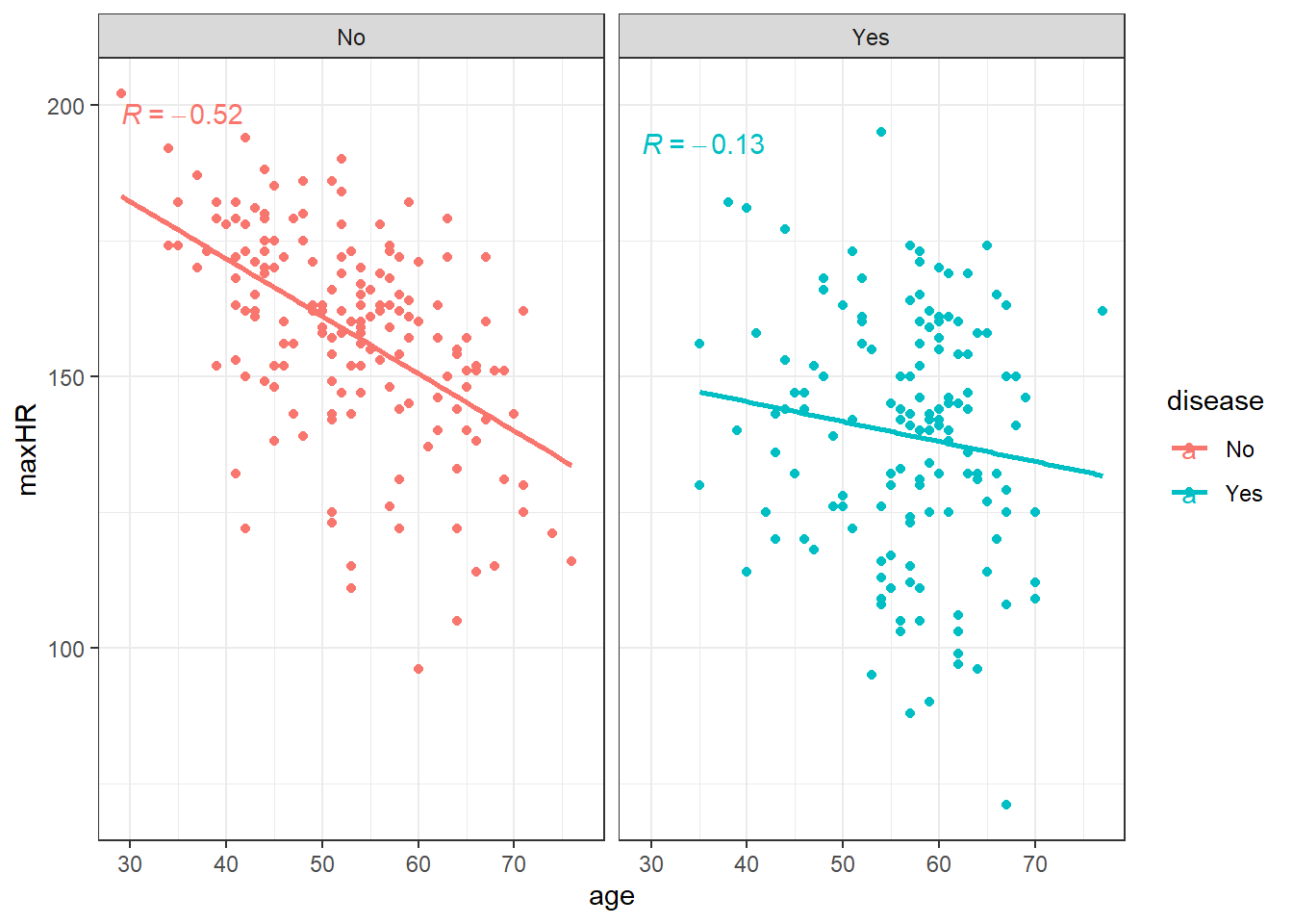
The guidelines from the Mayo Clinic apply mainly to the overall population of adults (age 16+).
This data is based on a study about heart disease.
Primarily, there are two groups in the data: those with heart disease, and those without.
Maybe heart disease has an effect.

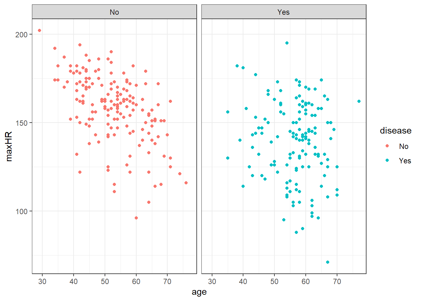
2.3.1.1 Grouping Means

2.3.2 Conditional Means vs Unconditional Means

Let’s concentrate on the formula for basic statistical models.

\[y = g(x) + \epsilon\]

2.3.2.1 Simplest Example

Unconditional Mean

\[y = \mu + \epsilon\]

2.3.2.2 Simple Model With Disease

\[y = 140 \pm 23\] Why might we use this model?

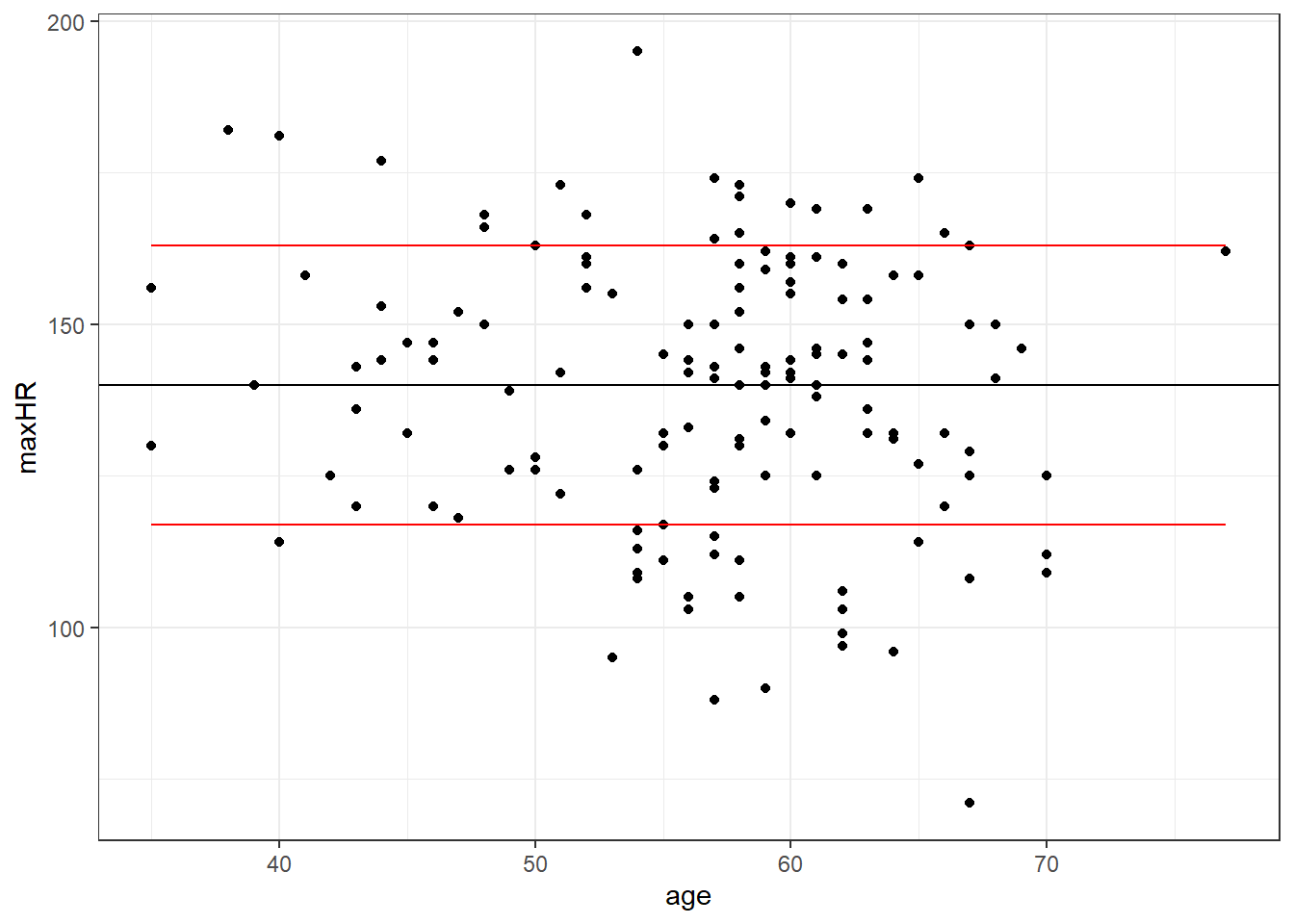
Percent 140 +/- 23
82.01439

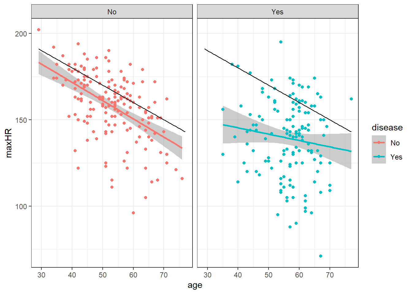
2.3.2.3 Model for Those Without Disease

The average maxHR should be about 214 - age, the standard deviation of that model is about 16

We denote this as:

\[y = 214 - x \pm 16\]

Percent 214 - x +/- 16
0.7256098

2.4 Linear models

2.4.1 Simple linear models: one predictor variable.

The simple linear model says the \(\mu_{y|x}\) is a line that depends on \(x\) based on a \(y\)-intercept which we denote by \(\beta_0\) and a slope which we denote \(\beta_1\).

\[\mu_{y|x} = \beta_0 + \beta_1 x\]

Conditional mean (deterministic)
\(\beta_0\): y-intercept
\(\beta_1\): slope

\[ y = \beta_0 + \beta_1 x + \epsilon = \mu_{y|x} + \epsilon \]

\(\epsilon\) is the error in the model (noted as “randomness” in some lecture videos¹)

2.4.2 Linear models with more than one predictor variable

A linear model in general means a model that can be written as a sum of variables and coefficients:

\[y = \beta_0 + \sum_{i=1}^k\beta_i x_i + \epsilon\]

\(\mu_{y | x}\) deterministic
\(\epsilon\) is the model error

\[ y = \beta_0 + \beta_1x_1 + \beta_2x_2 + \beta_3x_3 + ... + \beta_kx_k + \epsilon \]

2.5 Getting Started with Measuring Association

Let’s look back at that heart data.

2.6 Linear Correlation

We refer to the strength of relation between two variables to be their correlation. There are a few common ways to measure correlation. The most common is the following.

Pearson product-moment correlation:

\[ r = \frac{\sum_{i=1}^n {\left(X_i - \bar{X}\right)\left(Y_i - \bar{Y}\right)} }{ \sqrt{\sum_{i=1}^n {\left(X_i - \bar{X}\right)^2}\sum_{i=1}^n{\left(Y_i - \bar{Y}\right)^2}}} \]

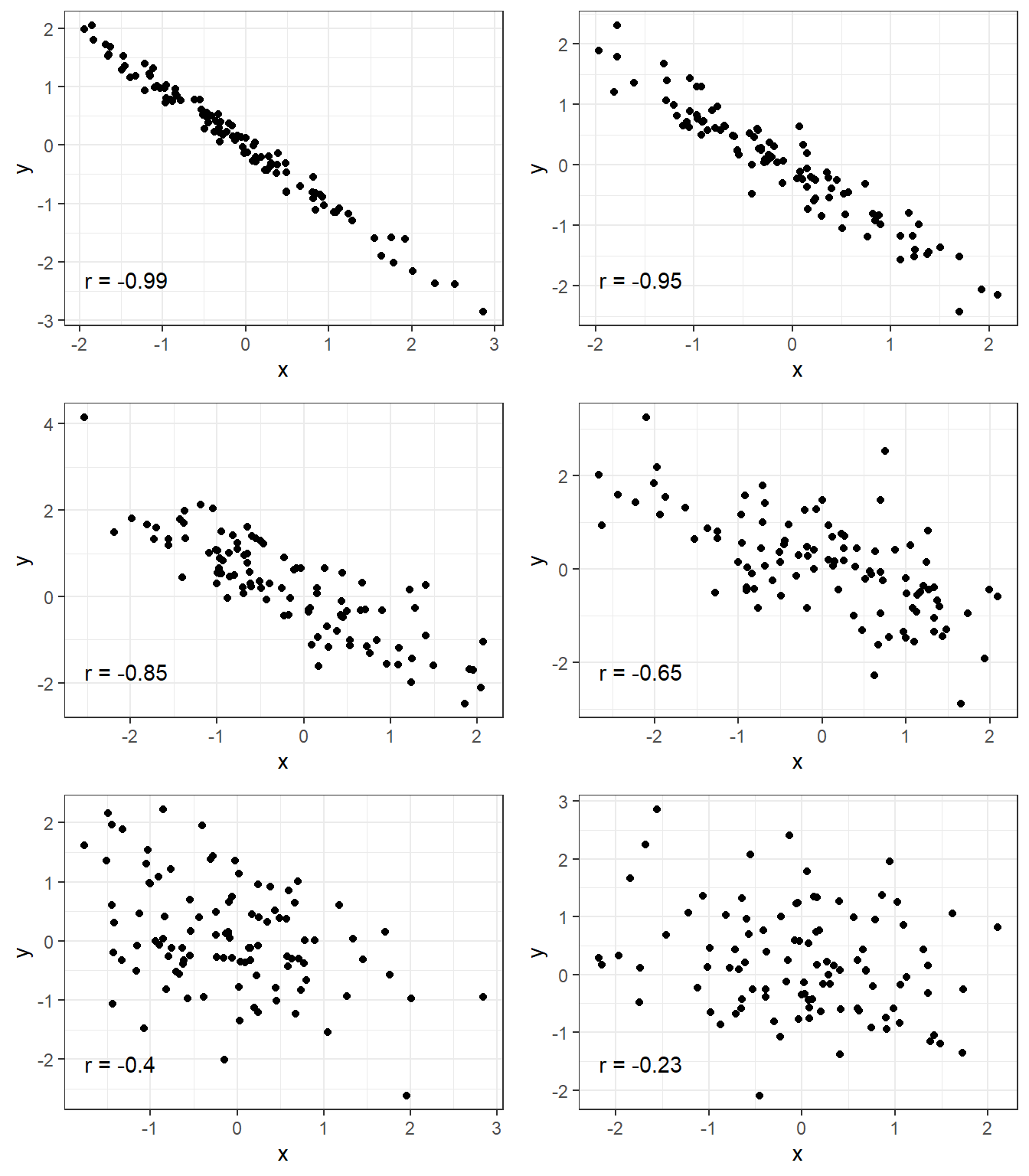
Here are some of the common properties of \(r\):

It can take on a value from -1 to 1.
If it is negative, then there is a “negative” relation between \(x\) and \(y\) which means as \(x\) increases, \(y\) decreases.
If it is positive, then there is a “positive” relation between \(x\) and \(y\) which means as \(x\) increases, \(y\) increases.
The closer to -1 or 1, the closer the \(x\) and \(y\) observations follow a straight line.
The above calculation is an estimate of what is the true correlation between two random variables/populations \(X\) and \(Y\).
This true correlation is denoted by \(\rho\)
Thus, \(r\) is a point estimate (remember that term?) of \(\rho\) (i.e., it is \(\hat \rho\)).

2.6.1 Correlation Strength Examples

2.6.2 Linear correlation of the heart data

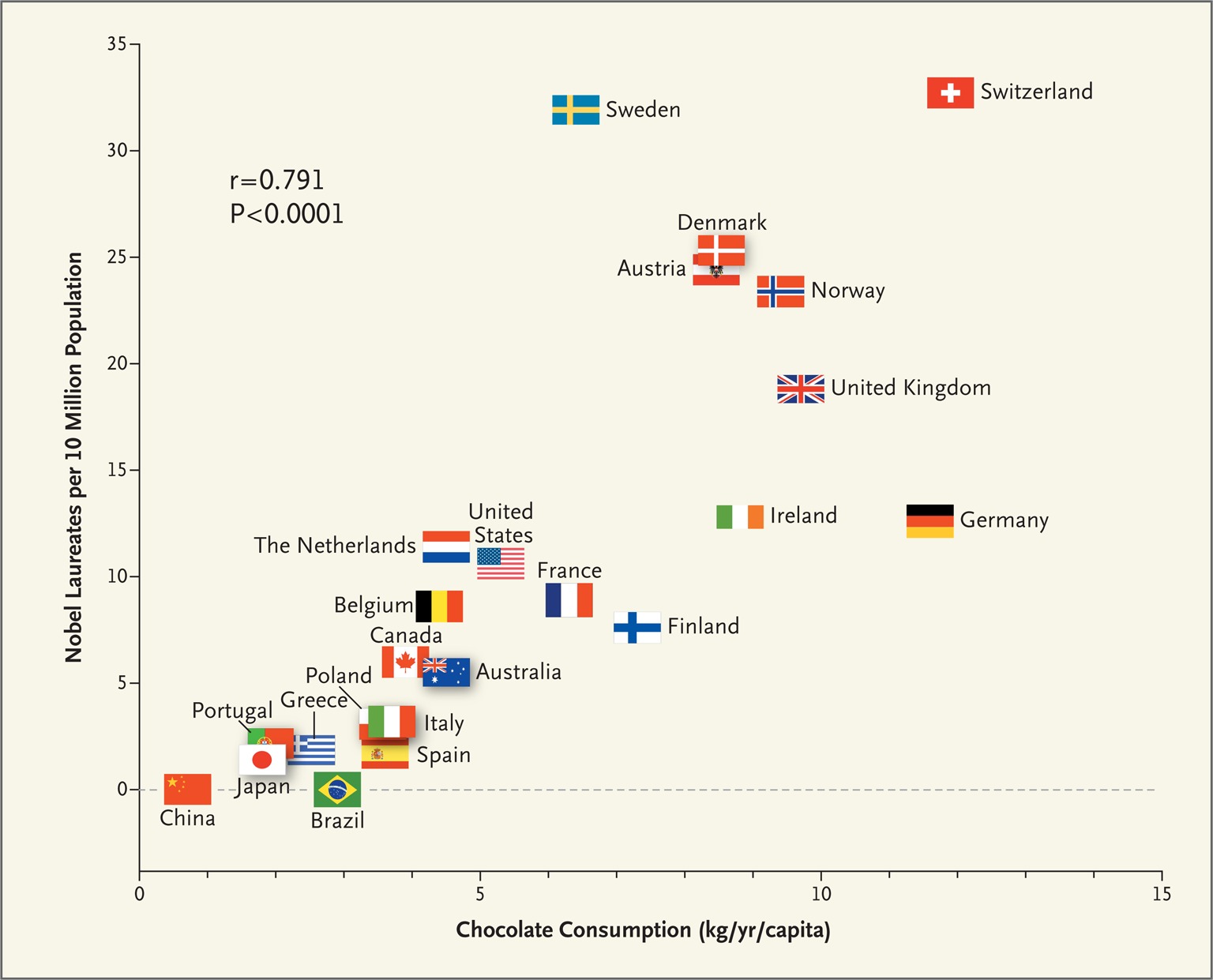
2.6.3 Correlation does not imply causation

Messerli, F. H. (2012). Chocolate Consumption, Cognitive Function, and Nobel Laureates. New England Journal of Medicine, 367(16), 1562-1564. doi:10.1056/nejmon1211064

The author tried to assert that this point towards the idea that chocolate increases cognitive function.

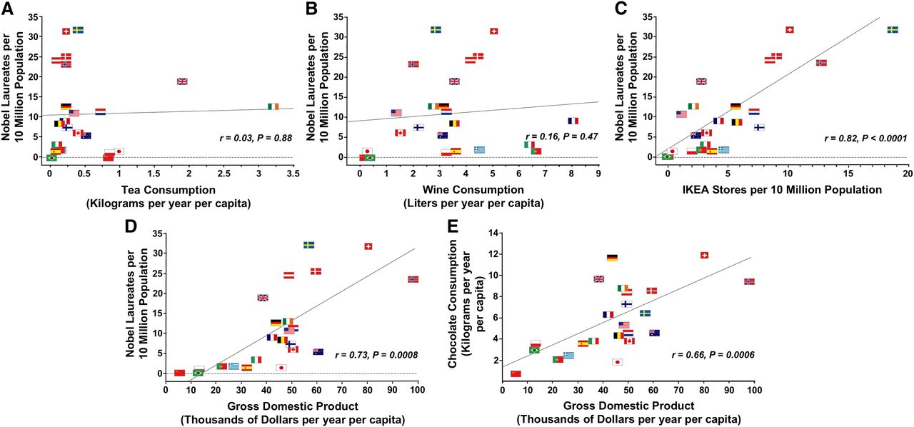
A rebuttal from various authors produced the following graphs. What might be in common?

2.6.4 cOrReLlAtIoN dOeS nOt ImPlY cAuSaTiOn

I feel like this is a fall back phrase for those that just want some sort of easy yes/no kind of answer. “It’s a correlation? Then this result is worthless.” This is incredibly lazy logic.

Do not dismiss correlations out of hand.
Use them to ask questions!
Correlation may not imply causation but it does imply a connection.
Finding the connection the cause of the non-cause would be quite interesting in a lot of scenarios.

Correlation \(\neq\) causation can be abused.

An article from the Science Based Medicine blog says:

“For example, the tobacco industry abused this fallacy to argue that simply because smoking correlates with lung cancer that does not mean that smoking causes lung cancer. The simple correlation is not enough to arrive at a conclusion of causation, but multiple correlations all triangulating on the conclusion that smoking causes lung cancer, combined with biological plausibility, does.”

It should be noted that other methods can, and should, be used to derive causation

2.7 Non-linear correlation

First, let’s look at a purely deterministic system.

pressure is vapor pressure of mercury in mm Hg. (pressure inside a closed system)
temperature is the temperature in \(^\circ C\).

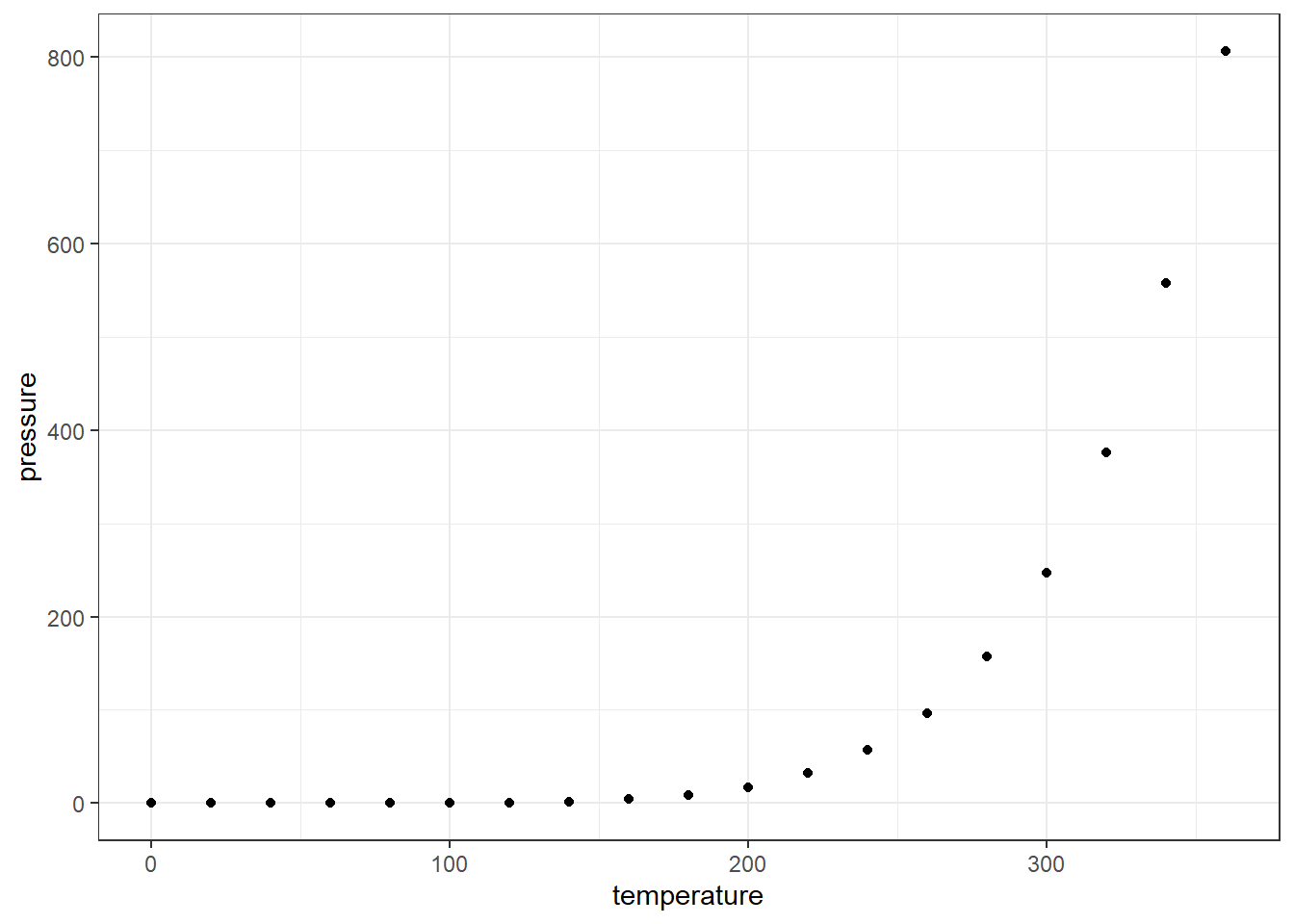
2.7.1 True Pressure Equation

How precise? Well here is the equation for calculating the vapor pressure of an element or molecule.

\[ P = 10^{\left( \displaystyle{A} - \dfrac{B}{C+T} \right)} \]

\(P\) is vapor pressure.
\(A\), \(B\), and \(C\) are constants based on the temperature scale, pressure scale, and element/molecule.
\(T\) is the temperature.

The NIST reports the constants for mercury when pressured is measured in bar and temperature is measured in Kelvin (K)

\(A = 4.85767\)
\(B = 3007.129\)
\(C = -10.001\)

Notice these are constants. No randomness here, no error here.

2.7.2 Using the Equation

Next, let’s plot the equation to our points.

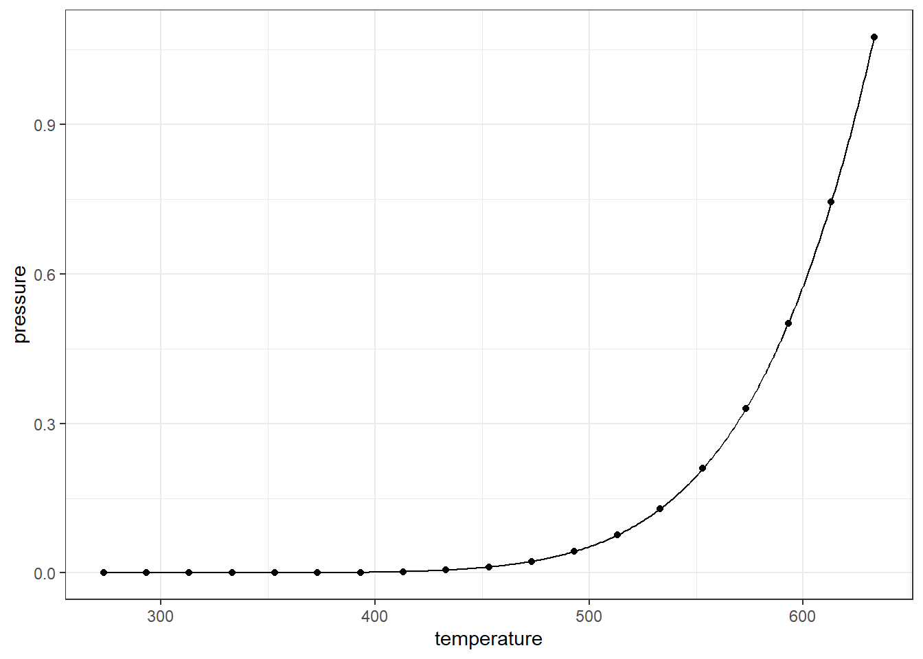
The relationship between vapor pressure and temperature seems to be perfectly accounted for by this equation. If we were to have a way to measure the strength of the relationshipo, it would hopefully reflect that perfect relation.

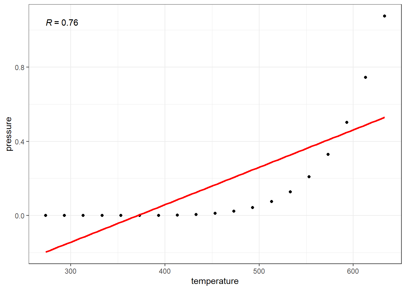
2.7.3 Using Transformations

\[P = 10^{\left( \displaystyle{4.85767} - \dfrac{3007.129}{-10.001+T} \right)}\]

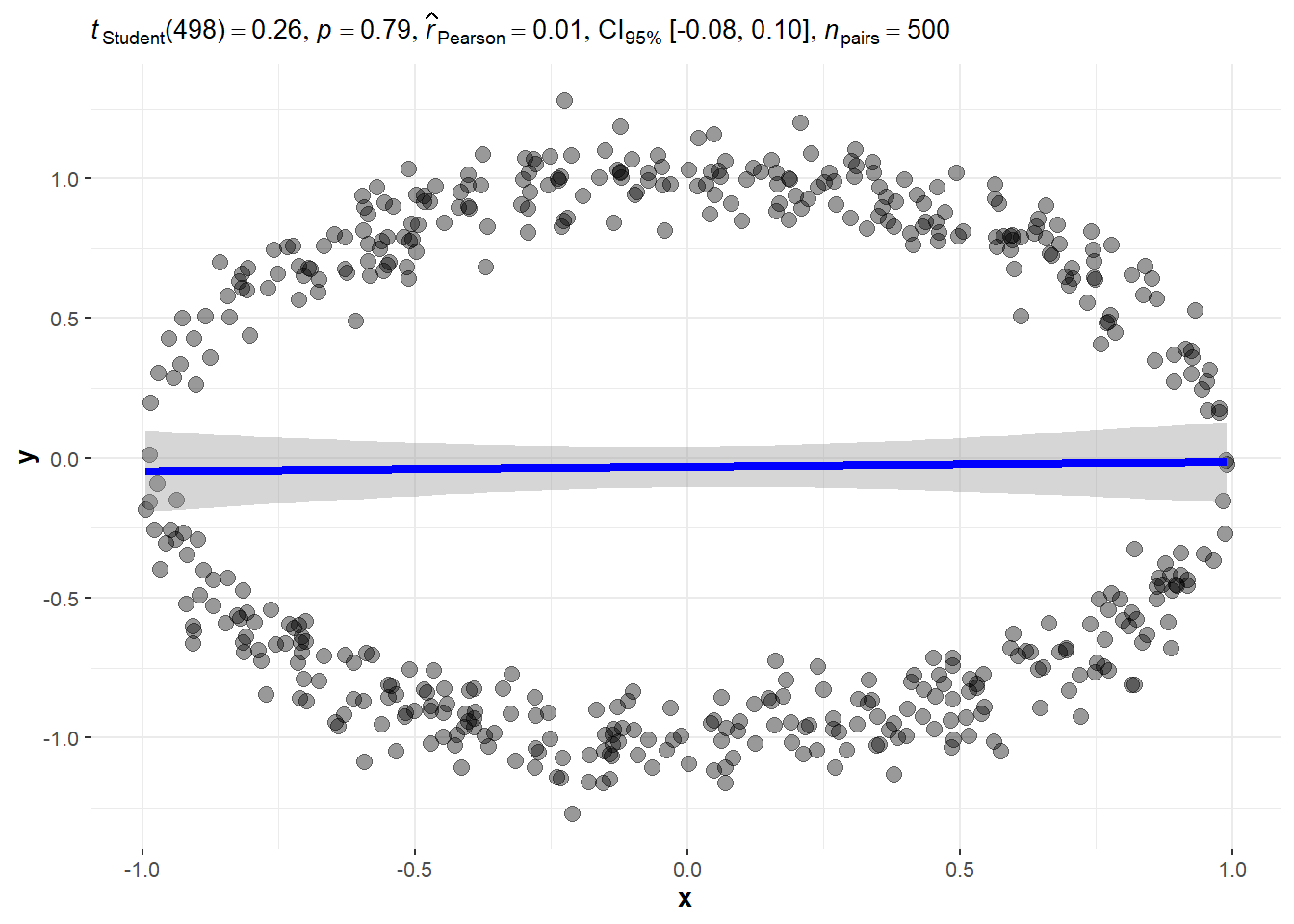
2.8 Zero Linear Relation Examples

Data falling on a circle. This is a “non-functional” relatioship. The mathematical definition of a function stipulates only one value of \(f(x)\) is the outcome for a value of \(x\). Another way of saying this is that one input value \(x\) should result in one and only one output value \(y\). (Remember that horizontal line rule?) On a circle, two values are possible for an input value of \(x\), except the leftmost and rightmost points of the circle.
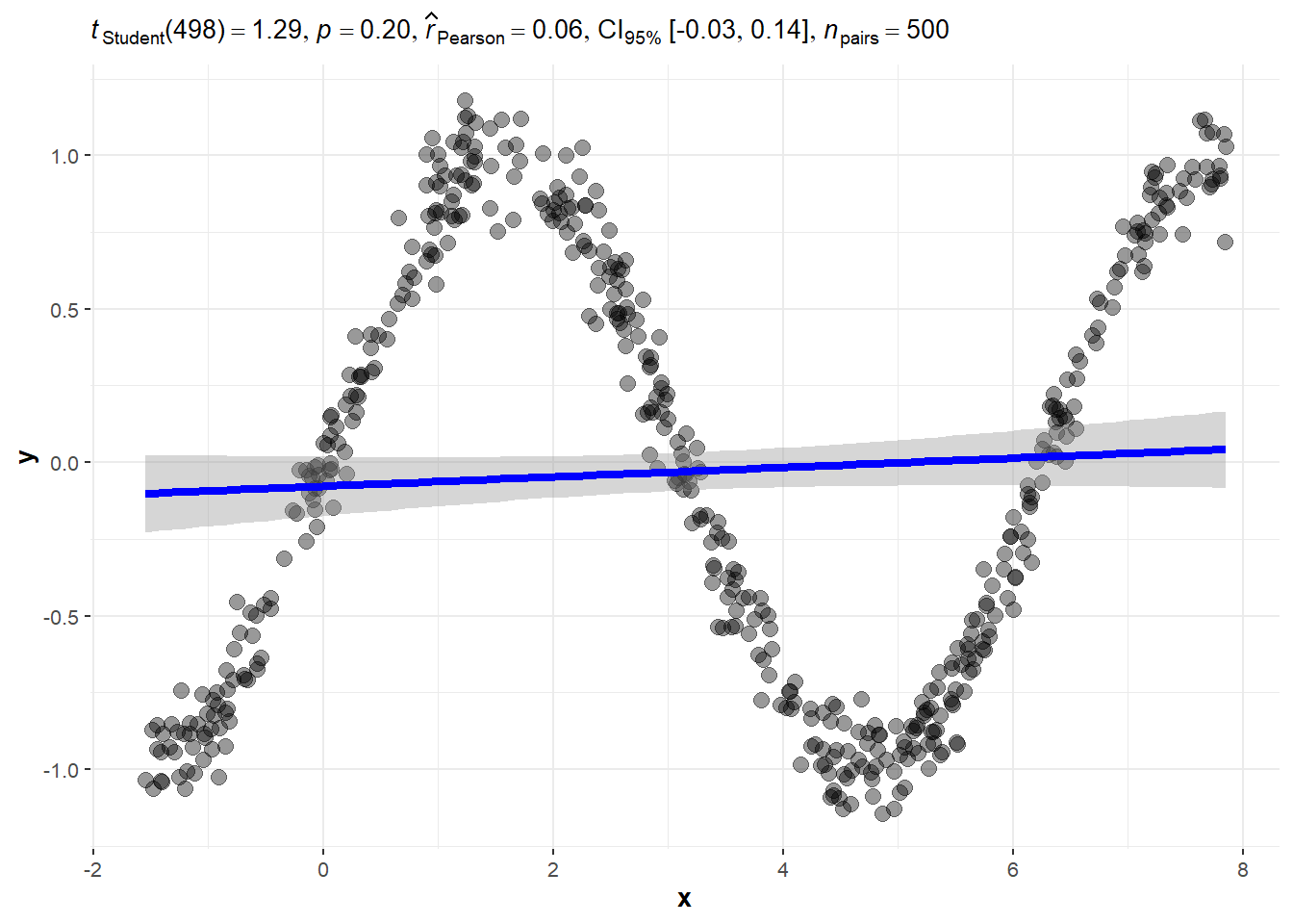
Data from a sine wave.
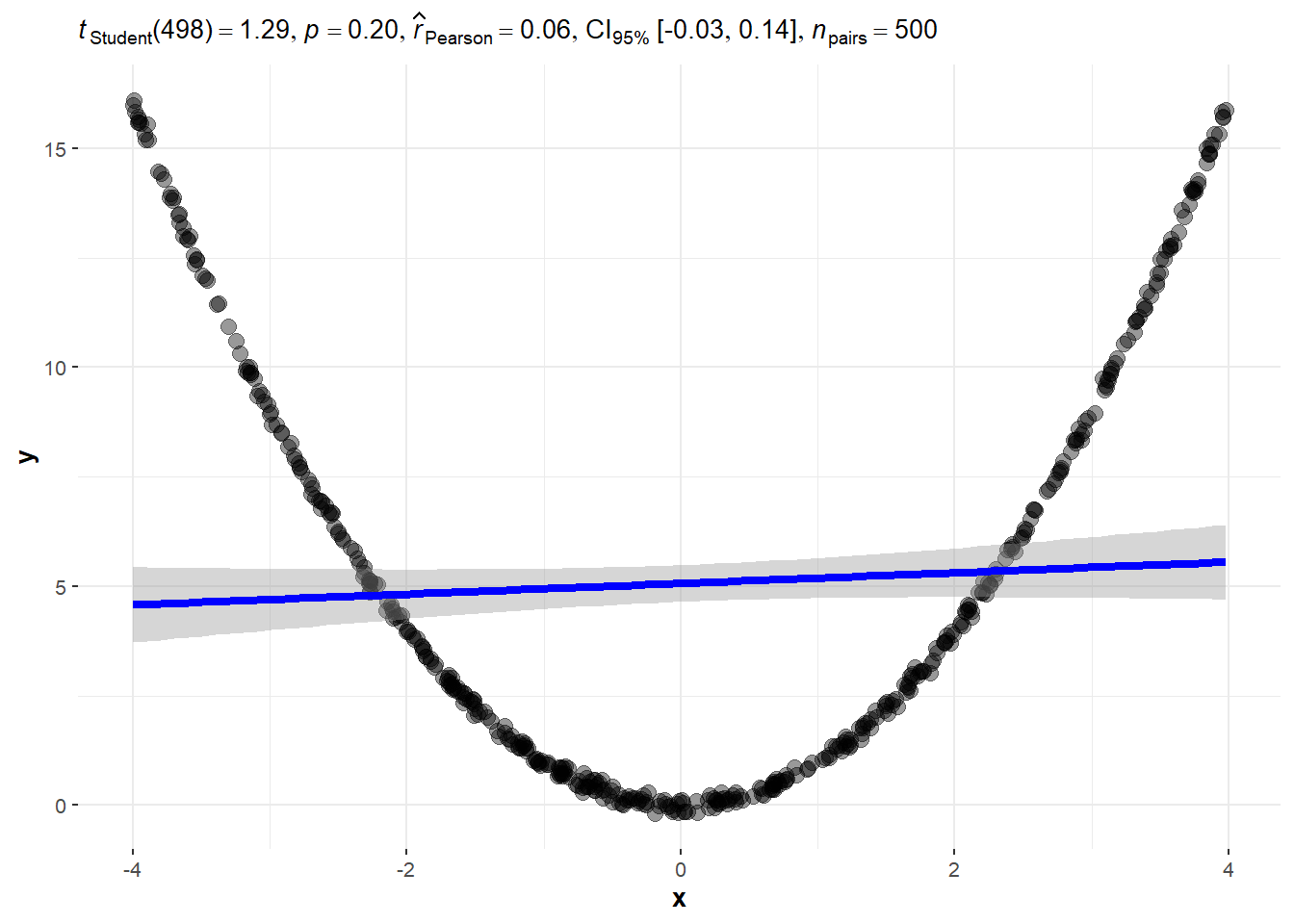
Data from a quadratic function.

2.8.1 Circle

2.8.2 Sine Wave

2.8.3 Quadratic

2.9 Kendall’s \(\tau\): A Correlation that identifies certain non-linear

Concordance: \((x_i-x_j)(y_i-y_j)\) is positive. The pair of points indicate a positive trend.

Discordance:\((x_i-x_j)(y_i-y_j)\) is negative. The pair of points indicate a negative trend.

\[\hat{\tau} = \frac{2}{n(n-1)}\sum_{i<j} sgn\left(x_i - x_j\right)sgn\left(y_i - y_j\right)\]

\[ sgn(x) = \begin{cases}1, \quad x > 0\\ -1, \quad x < 0\\ 0, \quad x = 0\end{cases} \]

Note: Kenall’s \(\tau\) should only be used for “monotonic” functions. Monotonic functions can only have an upward trend that is never downward, or vice versa. (Non-decreasing or non-increasing.)

Another Note: There are three commonly used versions of Kendall’s \(\tau\). This one is known as Tau-a. Tau-b should be used for data where there ties.

2.9.1 Alternative Expression for Kendall’s \(\tau\)

We can express Kendall’s \(\tau\) in a more intuitive way. Remember a pair of observations is \((x_i, y_i)\) and \((x_j, y_j)\).

Let \(n_c\) be the number of concordant pairs of observations.
Let \(n_d\) be the number of discordant pairs of observations.
Let \(N\) be the total number of possible unique pairs of observations.

\[\tau = \dfrac{n_c - n_d}{N}\] or

\[\tau = p_c - p_d\]

where

\(p_c\) is the proportion of times \(x\) and \(y\) increased together.
\(p_d\) is the proportion of times \(y\) decreased when \(x\) increased.

Note that \(N = \binom{n}{2} = \frac{n(n-1)}{2}\), where \(n\) is the number of observations.

This may make the interpretation a little more graspable.

\(p_c + p_d\) must equal \(1\). (And \(n_c + n_d\) must equal \(N\)). A consequence of this and the fact that \(\tau = p_c - p_d\)
- \(p_c = \frac{1 + \tau}{2}\)
- \(p_d = \frac{1 -\tau}{2}\)
When \(\tau\) is positive it is how much more often we see an concordance, i.e., \(x\) increases when \(y\) increases, compared to discordance where \(x\) increases and \(y\) decreases.
- If \(\tau = 0.5\) then \(p_c = 0.75\) and \(p_d = 0.25\). So 75% of the time \(y\) was increasing compared to 25% of the time
When \(\tau\) is negative its absolute value is how much more likely we are to see a decrease in \(y\) when \(x\) increases.
If \(\tau = - 0.7\) then \(p_c = 0.15\) and \(p_d = 0.85\), so 85% of the time we saw a decrease in \(y\) whereas only 15% of the time we saw an increase in \(y\)

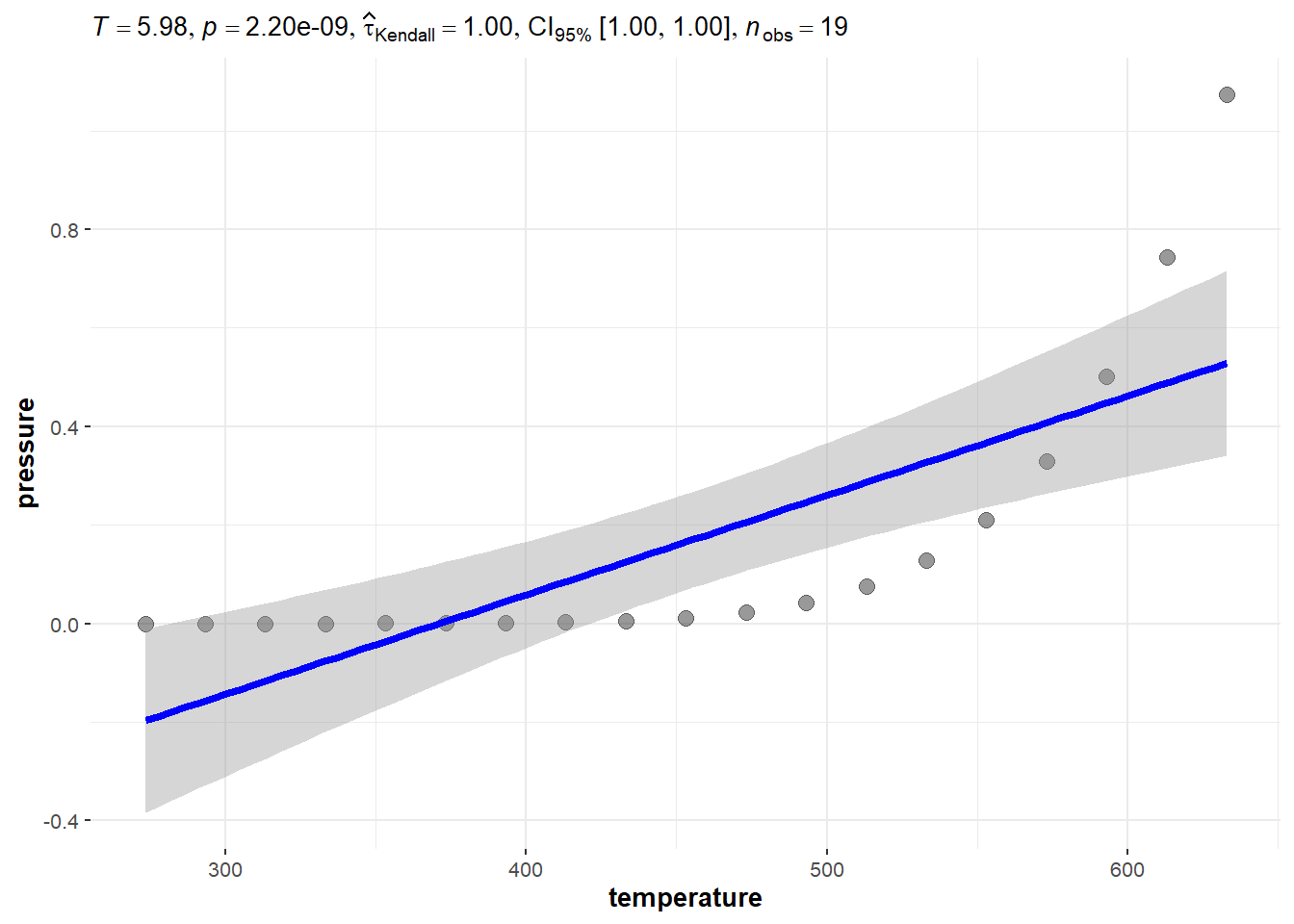
2.9.2 Kendall’s \(\tau\) with the pressure data

Recall the vapor pressure example.

2.9.3 Kendall’s \(\tau\) on some mice proteins data

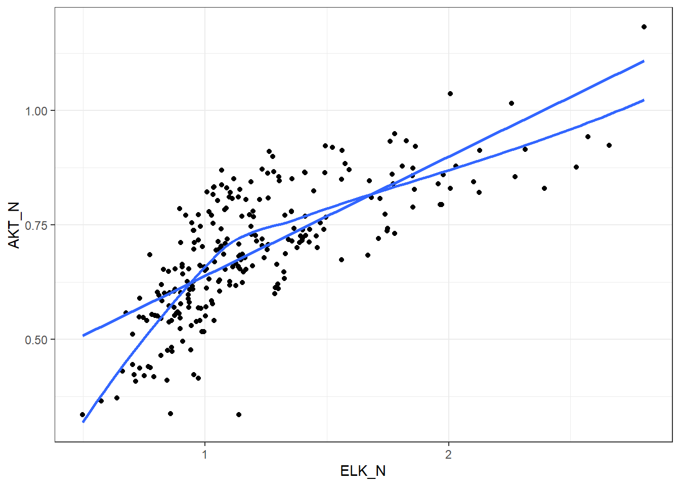
KendallCorr numeric	0.5866605
PearsonCorr numeric	0.7394402

2.9.4 A transformation

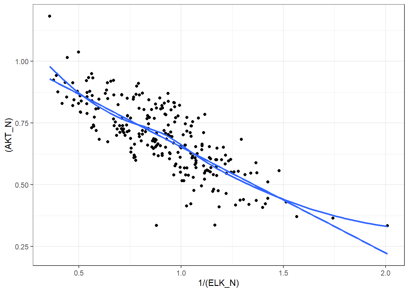
KendallCorr numeric	-0.5866605
PearsonCorr numeric	-0.7865069

2.9.4.1 Monotonic

Definition: In the context of a sequence of numbers, “monotonic” means the sequence is either always increasing or always decreasing. It moves in one direction, without changing direction.
Explanation: Think of a monotonic sequence like walking up or down a staircase. You’re either consistently going upwards (increasing) or consistently going downwards (decreasing). You never switch directions and go up and then down, or down and then up.

Examples:

Monotonic Increasing: 2, 5, 8, 11, 15 (each number is larger than the one before it)
Monotonic Decreasing: 10, 7, 4, 1, -2 (each number is smaller than the one before it)
Not Monotonic: 3, 6, 4, 8 (it increases, then decreases, so it’s not monotonic)

Monotonic Transformation

Definition: A monotonic transformation is a way of changing a set of numbers into a different set of numbers, but in a way that preserves the order of the original set.
Explanation: Imagine you have a line of people arranged from shortest to tallest. A monotonic transformation would be like giving everyone in line platform shoes. Everyone gets taller, but the order from shortest to tallest stays the same.

Examples:

Original sequence: 2, 5, 8
- Monotonic transformation (adding 3 to each number): 5, 8, 11
- Monotonic transformation (multiplying each number by 2): 4, 10, 16

Why is this important in statistics?

Monotonic transformations are useful in statistics because they can sometimes simplify data analysis without changing the fundamental relationships within the data. For instance, they can be used to:

Make data easier to work with: Transforming data can sometimes make it easier to visualize or analyze.
Meet the assumptions of statistical tests: Some statistical tests require data to have certain properties. Monotonic transformations can sometimes help data meet those assumptions.

Key takeaway: Monotonic means “always going in one direction.” A monotonic transformation changes the values in a dataset but keeps the order the same.

We should ↩︎