6  Module 6: ANOVA and Experimental Design

6.1 One-Way ANOVA

Here are some code chunks that setup this chapter.

# Here are the libraries I used
library(tidyverse) # standard
library(knitr) # need for a couple things to make knitted document to look nice
library(readr) # need to read in data
library(ggpubr) # allows for stat_cor in ggplots
library(ggfortify) # Needed for autoplot to work on lm()
library(gridExtra) # allows me to organize the graphs in a grid
library(car) # need for some regression stuff like vif
library(GGally)

# This changes the default theme of ggplot
old.theme <- theme_get()
theme_set(theme_bw())

Comparing More Than Two Group Means: Analysis of Variance (ANOVA or AOV)

6.1.1 Review: Comparing Two Groups (Sections 7.1 - 7.7 of JB Statistics)

Two-Sample Tests

\(H_0: \mu_1 = \mu_2\)

\(H_1: \mu_1 \neq \mu_2\)

6.1.1.1 The two-sample t-test: Pooled

Student’s two-sample \(t\)-test, and assumes unknown but equal population variances/standard deviations, i.e.,\(\sigma_1 = \sigma_2\).

We use a pooled sample variance estimate:

\[ s_p^2 = \frac{(n_1-1)s_1^2 + (n_2 - 1)s_2^2}{(n_1-1)+(n_2-1)} \]

\[ t = \frac{\bar{y_1}-\bar{y_2}}{\sqrt{s_P^2\left(\frac{1}{n_1}+\frac{1}{n_2}\right)}} \]

And the degrees of freedom is \(df = n_1 + n_2-2\)

• Pro: Powerful if \(\sigma_1 = \sigma_2\).

• Con: When is that true?

6.1.1.2 Welch’s two-sample t-test

Assume \(\sigma_1 \neq \sigma_2\) \[ t = \frac{\bar{y_1}-\bar{y_2}}{\sqrt{\frac{s_1^2}{n_1}+\frac{s_2^2}{n_2}}} \]

\[ df = \frac{\left(\frac{s_1^2}{n_1}+\frac{s_2^2}{n_2}\right)^2}{\frac{\left(s_1^2/n_1\right)^2}{n_1-1}+\frac{\left(s_2^2/n_2\right)^2}{n_2-1}} \]

6.1.1.3 R command, t.test()

t.test(x, y)

By default, this performs Welch’s test. If you must perform Student’s test:

t.test(x, y, var.equal=TRUE)

6.1.1.4 Hypothetical Example: Three Groups

Let’s consider having three groups.

• In the code below, the groups are generated and technically we know the populations means.

• But we will only have the sample data in reality.

• How can we use three sample means at once to distinguish between three groups?

n = 200

data <- data.frame(x = rnorm(n, 0, 1), 
                   y = rnorm(n, 1, 1), z = rnorm(n, 2, 1))
data <- gather(data, key = 'group', value = 'response')

# sample means

sample.means <- aggregate(x = response ~ group , 
                          data = data, FUN = mean)
sample.means$mu = c(0,1,2)

ggplot(data, aes(x = response, y = after_stat(density), 
                 color = group, fill = group)) + 
  geom_density(alpha = 0.5) + 
  geom_vline(data = sample.means, aes(xintercept = response, 
                                      color = group))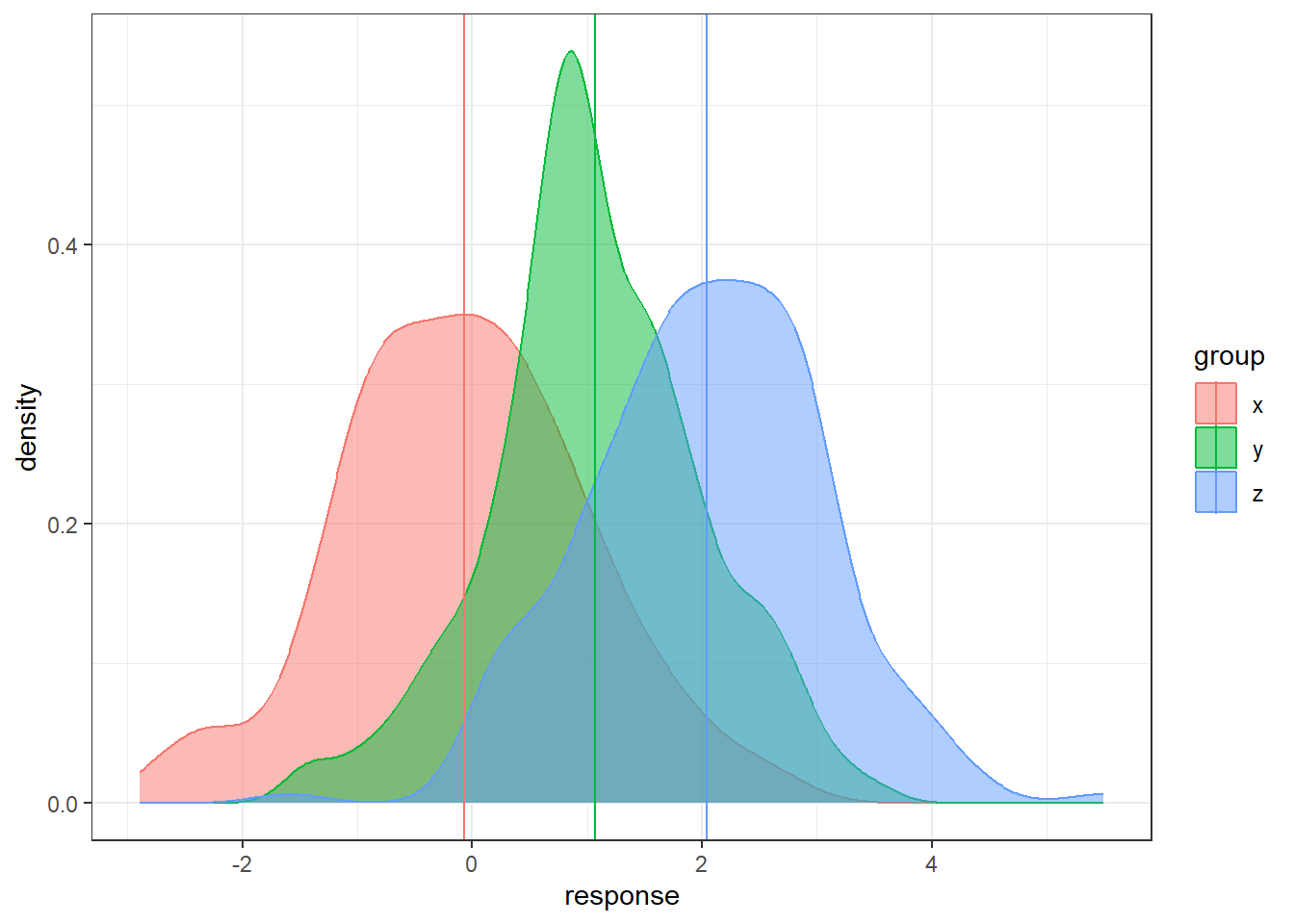

There is sampling variability associated with each sample mean. Run this code a few times do see how much the sample means will change from sample to sample. How do we account for the sampling variability when comparing three groups simultaneously? How do we even compare three groups simultaneously?

6.1.2 Analysis of Variance

6.1.2.1 General Objective of Analysis of Variance (ANOVA)

First, we are going to have a hypothesis test involved with comparing several groups.

• The null hypothesis is going to be the similar to before, all the groups have equivalent population means.

• The alternative is a bit trickier…

Hypotheses:

\(\begin{aligned} H_0&: \mu_1 = \mu_2 = \dots = \mu_t\\ H_1&: \text{not that...} \end{aligned}\)

Why not just do a bunch of separate t-tests?

If we have three groups:

• Compare group 1 to group 2.
• Compare group 1 to group 3.
• Compare group 2 to group 3.

And that would account for all possible pairings of groups. However, each of these would be a separate hypothesis test.

These are called pair-wise comparisons.

In general, if there are \(t\) groups, there are

\[\binom{t}{2} = \frac{t(t-1)}{2}\]

unique pair-wise comparisons.

6.1.2.2 Familywise Error Rate: What happens when you do multiple hypothesis tests

Say we had four treatment groups and we wanted to compare the means of all four groups to see if any differed.

Through pairwise comparisons, we would end up with \(\frac{4\cdot 3}{2} = 6\) total comparisons.

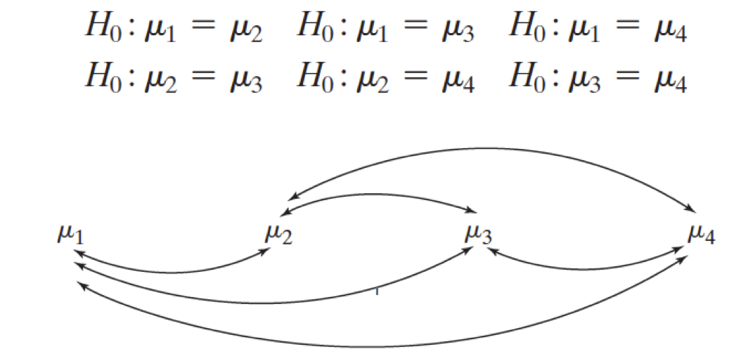
This would amount to 6 hypothesis tests to decide which if any group means differ.

• Assume each hypothesis test is done with the same Type I Error Rate \(\alpha\).
  • Pr(Reject \(H_0\) | \(H_0\) True)
• This is known as a family of hypothesis tests, a set of hypothesis tests under one objective.
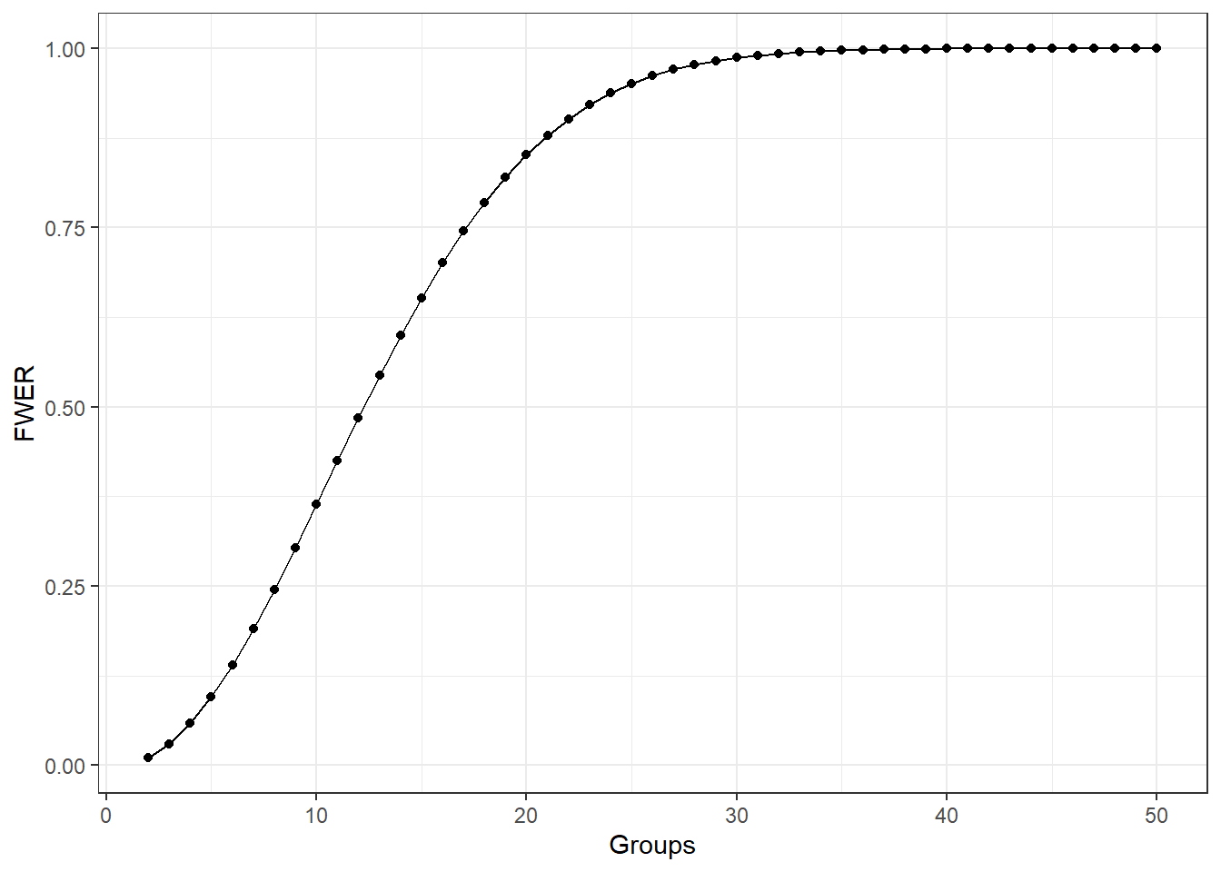
• The Family Wise Error Rate (FWER) is the probability of making at least one Type I Error among a family of hypothesis tests.

\[\begin{aligned} FWER & = 1 - (1 - \alpha)^c \\ &> \alpha \text{ for } c = 2, 3, \dots \end{aligned}\]

The following graph shows what happens to the FWER when the number of groups increases and each pairwise comparison done with \(\alpha = 0.01\).

6.1.2.3 How ANOVA Works

The analysis of variance (ANOVA) is just that. It looks at two types of variability in the data.

• Between or Treatment Variability: This is the variability between the groups which is measured by essentially computing a the variance of the sample means between the different groups.

• The Within or Error Variability: This is a collective measure of the variability within the groups.

If the Between/Treatment Variability is noticeably larger than the the Within/Error variability, we have strong evidence in favor that the least some groups have different population means.

6.1.2.4 Treatment versus Error Variability Demos

Here is a simulated dataset with moderately small within/error variability relative to the between/treatment variability

n = 200

data <- data.frame(x = rnorm(n, 0, 1),
                   y = rnorm(n, 1, 1), z = rnorm(n, 2, 1))
data <- gather(data, key = 'group', value = 'response')

sample.means <- aggregate(x = response ~ group , 
                          data = data, FUN = mean)
sample.means$mu = c(0,1,2)

ggplot(data, aes(x = response, y = after_stat(density), 
                 color = group, fill = group)) + 
  geom_density(alpha = 0.5) + 
  geom_vline(data = sample.means, aes(xintercept = response, 
                                      color = group))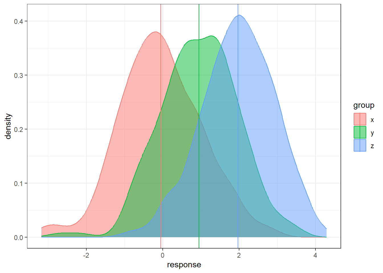

Here is an example a very small within/error variability relative to the between/treatment variability.

n = 200

data <- data.frame(x = rnorm(n, 0, 0.1),
                   y = rnorm(n, 1, 0.1), z = rnorm(n, 2, 0.1))
data <- gather(data, key = 'group', value = 'response')

# sample means

sample.means <- aggregate(x = response ~ group , 
                          data = data, FUN = mean)
sample.means$mu = c(0,1,2)

ggplot(data, aes(x = response, y = ..density.., 
                 color = group, fill = group)) + 
  geom_density(alpha = 0.5) + 
  geom_vline(data = sample.means, aes(xintercept = response, 
                                      color = group))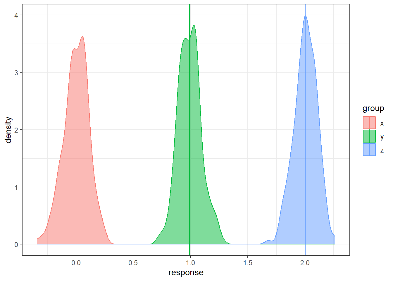

Lastly, large within/error variability relative to between/treatment variability.

n = 200

data <- data.frame(x = rnorm(n, 0, 5), 
                   y = rnorm(n, 1, 5), z = rnorm(n, 2, 5))
data <- gather(data, key = 'group', value = 'response')

# sample means

sample.means <- aggregate(x = response ~ group , 
                          data = data, FUN = mean)
sample.means$mu = c(0,1,2)

ggplot(data, aes(x = response, y = ..density.., 
                 color = group, fill = group)) + 
  geom_density(alpha = 0.5) + 
  geom_vline(data = sample.means, aes(xintercept = response, 
                                      color = group))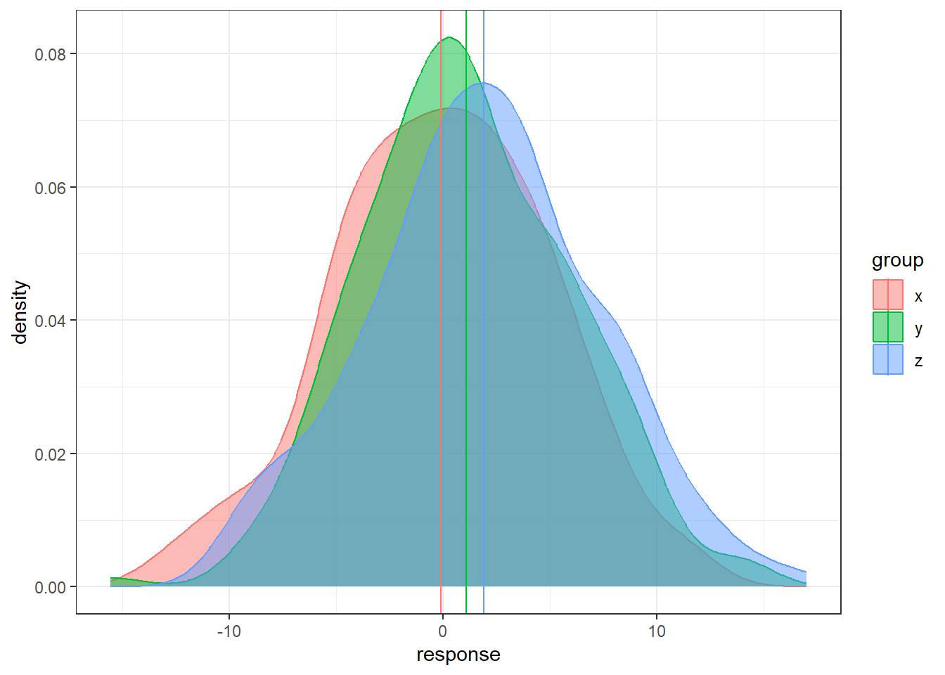

• In each situation, the population means are the same: 0, 1, and 2.
• In some situations it’s much easier to distinguish the groups than in others.

6.1.3 Formulating ANOVA: Notation

• \(y_{ij}\) is the \(j^{th}\) observation in the \(i^{th}\) treatment group.

  • \(i = 1, \dots, t\), where \(t\) is the total number of treatment groups.
  • \(j = 1, \dots, n_i\) where \(n_i\) is the number of observations in treatment group \(i\).

• \(\overline{y}_{i.} = \sum_{j=1}^{n_i}\frac{y_ij}{n_i}\) is the mean of treatment group \(i\).

• \(\bar{y}_{..} = \sum_{i=1}^{t} \sum_{j=1}^{n_i}\frac{y_{ij}}{N}\) is the over all mean of all observations.

  • \(N\) is the total number of observations.

6.1.3.1 Sums of Squares

Sum of Squares for the treatments

\(\begin{aligned} SST &= \sum_{i=1}^{t} n_i \left(\overline{y}_{i.} - \bar{y}_{..}\right)^2 \end{aligned}\)

Sum of squares for the errors

\(\begin{aligned} SSE &= \sum_{i=1}^{t} \sum_{j=1}^{n_i}\left(y_{ij} - \bar{y}_{i.}\right)^2 \end{aligned}\)

With each sum of squares, there is an associated degrees of freedom.

• Treatment: \(df_t = t-1\)
• Error: \(df_e = N - t\)

6.1.3.2 Mean Squares

\(\begin{aligned} MST &= \frac{SST}{t-1} \end{aligned}\)

\(\begin{aligned} MSE &= \frac{SSE}{N-t} \end{aligned}\)

6.1.3.3 Test Statistic

\(\begin{aligned} F_t = \frac{MST}{MSE}. \end{aligned}\)

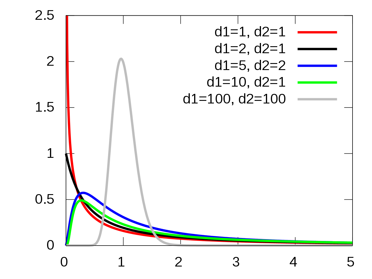
6.1.3.4 F-Distribution

Under the the following assumptions:

1. The null hypothesis is true, i.e., all groups have equivalent means,
2. The groups are indendent and normally distributed,
3. The groups all have equivalent variances,

the test statistic \(F_t\) follows an \(F(t-1, N-t)\) distribution.

6.1.3.5 F-Distribution Visualization

6.1.4 How is this a “Linear Model”

6.1.4.1 Means Model

Means Model:

\(\begin{aligned} y &= \mu_i + \epsilon \end{aligned}\)

Which leads to the hypotheses in ANOVA:

\(H_0: \mu_{1} = \dots = \mu_{t}\)

\(H_1\): The means are not all equal.

6.1.4.2 Effects Model

Effects Model:

\(\begin{aligned} y &= \mu + \tau_i + \epsilon \end{aligned}\)

The \(\tau_i\)’s are the shift parameters that cause the groups to differ.

Which leads to an equivalent set of hypotheses:

\(H_0: \tau_{1} = \dots = \tau_{t} = 0\)

\(H_1: \text{Not } H_0\)

6.1.5 OASIS MRIs

Variables in OASIS data

• Group: whether subject is demented, nondemented, or converted.
• Visit: (Not relevant) which visit number of the MRI
• Gender: M or F
• MR Delay: (Not relevant) time between each successive MRI. First MRIs
• Hand: Handedness of subject. All patients were R (right-handed)
• Age: Age in years
• Educ: Years of education
• SES: Socioeconomic status 1 - 5, low to high SES (arbitrary cutoffs most likely)
• MMSE: Mini Mental State Examination
• CDR: Clinical Dementia Rating, 0 - 2. 0 is non-dementia, CDR > 0 is severity of dementia.
• eTIV: Estimated Total Intracranial Volume (milliliters?)
• nWBV: Normalized Whole Brain Volume; Brain volume is normalized by intercranial volume to put subjects of different sizes and gender on the same scale. To my best knowledge…
• ASF: Atlas Scaling Factor; I tried investigating this but that’s some rabbit hole that is very deep apparently. It has something to do with the normalization I think.

Unlike before, we’re going to compare all three patient groups in the OASIS data: Demented, Nondemented, and Converted.|

Converted patients are those that entered the study that were no diagnosed with dementia, and then by the time the study ended they had been diagnosed with dementia.

The objective is to assess the Normalized Whole Brain Volume nWBV of the different groups and see if the mean nWBV differs.

oasis <- read_csv(here::here("datasets",'oasis.csv'))

6.1.5.1 Examining the data

Let’s look at the nWBVs overall.

nWBVmean <- mean(oasis$nWBV)

### geom_density() produces a "smoothed" histogram.
### if you wanted a histogram, you could use geom_histogram()


ggplot(oasis, aes(x = nWBV)) + 
  geom_density(fill = "lavender") +
  geom_vline(xintercept = nWBVmean)

Now let’s look at the grouped data.

# Get group means
## You can ignore this...
ybars <- aggregate(x = nWBV ~ Group, data = oasis, 
                   FUN = mean)



ggplot(oasis, aes(x = nWBV, color = Group, 
                  fill = Group)) + 
  geom_density(alpha = 0.1) +
  geom_vline(data = ybars, aes(xintercept = nWBV, 
                               color = Group))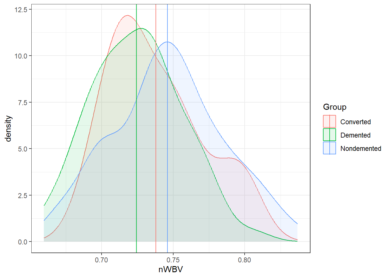

### When comparing groups, a standard way is to use boxplots.
ggplot(oasis, aes(y = nWBV, color = Group, 
                  x = Group)) + 
  geom_boxplot()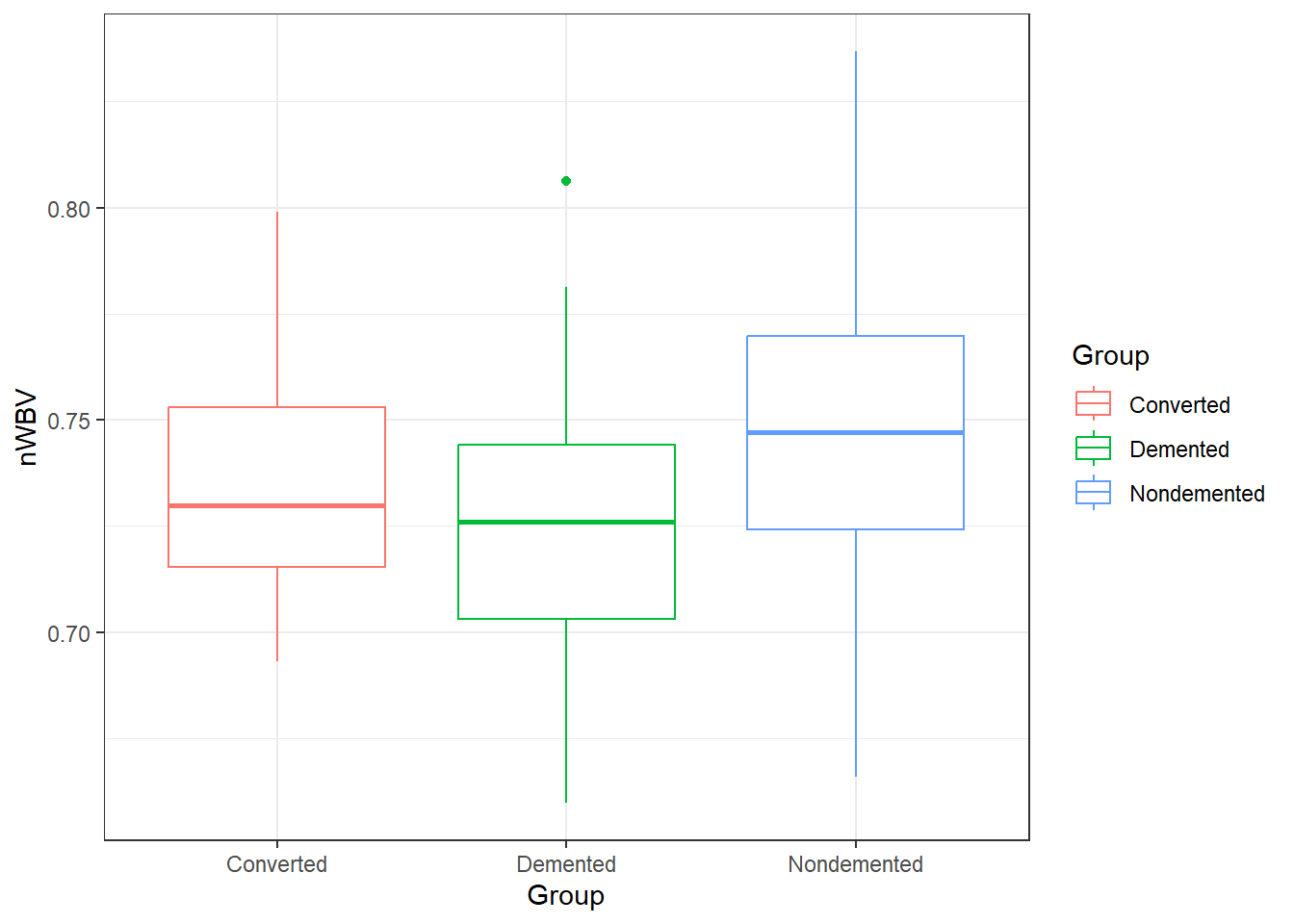

6.1.5.2 ANOVA in R: its lm() again

There are a few ways to do ANOVA in R. The approach that is most adaptable is to use the lm() function.

lm(formula = y ~ x, data)

So we create a linear model with nWBV as y and Group as x.

fit.lm <- lm(nWBV ~ Group, data = oasis)

In general, on lm objects we use the summary() function.

summary(fit.lm)

Call:
lm(formula = nWBV ~ Group, data = oasis)

Residuals:
      Min        1Q    Median        3Q       Max 
-0.080200 -0.022459  0.000674  0.023080  0.090780 

Coefficients:
                  Estimate Std. Error t value Pr(>|t|)    
(Intercept)       0.737860   0.009421  78.317   <2e-16 ***
GroupDemented    -0.013503   0.010401  -1.298    0.196    
GroupNondemented  0.008202   0.010297   0.797    0.427    
---
Signif. codes:  0 '***' 0.001 '**' 0.01 '*' 0.05 '.' 0.1 ' ' 1

Residual standard error: 0.03525 on 147 degrees of freedom
Multiple R-squared:  0.0806,    Adjusted R-squared:  0.06809 
F-statistic: 6.443 on 2 and 147 DF,  p-value: 0.002078

This technically contains all the information we need. Specifically look at the bottom of the summary where there is information on the F-statistic, degrees of freedom and p-value.

To get this information displayed in a more traditional format for an ANOVA, use theanova() function on an lm object.

anova(fit.lm)

Analysis of Variance Table

Response: nWBV
           Df   Sum Sq   Mean Sq F value   Pr(>F)   
Group       2 0.016014 0.0080069  6.4431 0.002078 **
Residuals 147 0.182677 0.0012427                    
---
Signif. codes:  0 '***' 0.001 '**' 0.01 '*' 0.05 '.' 0.1 ' ' 1

6.1.5.3 Alternative: aov()

An alternative is to use the aov() function in the same way:

fit.aov <- aov(nWBV ~ Group, data = oasis)

For an aov object, just use the summary() function to get results in a similar manner.

summary(fit.aov)

             Df  Sum Sq  Mean Sq F value  Pr(>F)   
Group         2 0.01601 0.008007   6.443 0.00208 **
Residuals   147 0.18268 0.001243                   
---
Signif. codes:  0 '***' 0.001 '**' 0.01 '*' 0.05 '.' 0.1 ' ' 1

In any of these cases, we have very strong discrepancy with null model (i.e., all means are equal) for a different mean nWBV between the different groups of patients.

6.1.5.4 Statistical Versus Practical Significance

Let’s look back at the nWBVs split by group:

ggplot(oasis, aes(x = nWBV, color = Group, 
                  fill = Group)) + 
  geom_density(alpha = 0.10) +
  geom_vline(data = ybars, aes(xintercept = nWBV, 
                               color = Group))

And here are the means of each group.

# This is some tidyverse magic.

oasis %>% 
  group_by(Group) %>%
  summarise(mean = mean(nWBV))

# A tibble: 3 × 2
  Group        mean
  <chr>       <dbl>
1 Converted   0.738
2 Demented    0.724
3 Nondemented 0.746

# Or using the model using modelbased

library(modelbased)
fit.aov %>%
  estimate_means()

Estimated Marginal Means

Group       | Mean |       SE |       95% CI | t(147)
-----------------------------------------------------
Converted   | 0.74 | 9.42e-03 | [0.72, 0.76] |  78.32
Demented    | 0.72 | 4.41e-03 | [0.72, 0.73] | 164.38
Nondemented | 0.75 | 4.15e-03 | [0.74, 0.75] | 179.58

Variable predicted: nWBV
Predictors modulated: Group

Among the groups, the biggest difference in means between the demented and non-demented group is about 0.02.

Is that a big difference?

• Statistically, it is with \(p = .0021\).
• On a relative scale it is about a 3% difference.
  • Is this a practical difference, i.e., does it matter?
  • That would be very dependent on the field, the research question, the researcher, the impacts, and so on…
  • What is an important difference is a specific matter that should be discussed and defined.

6.1.6 Multiple Comparisons

Suppose we did a single test between two group means:

We would have: \[ t = \frac{\overline{y_i}-\overline{y_j}}{SE_{\overline y_i - \overline y_j}} \] Then we get a p-value based on that t-distribution with some degrees of freedom defined by the method we were using for the comparison, e.g., equal or unequal variance two-sample t-test, ANOVA, and others…

Null Hypothesis Significance Testing (NHST) Approach

In NHST we “Reject \(H_0\) if \(p \le \alpha\).

• \(\alpha\) is the Type I error rate: “The probability of rejecting \(H_0\) when \(H_0\) is true.”

  • This would be a “false positive” or a “false discovery”

P-value as a spectrum.

• We would talk about the strength of evidence for declaring \(\mu_i - \mu_j\).

  • This approach would not have a Type I error per se.
  • The idea of a Type I error would fall on a spectrum as well.

6.1.7 Multiple testing problem

In the ANOVA setting, should we Reject \(H_0\) (all means are equal), or declare the strength of evidence is sufficient to be confident of a difference.

• The next step is to look and see which specific groups/means differ.

• This involves pairwise comparisons.

\[ t = \frac{\overline{y_i}-\overline{y_j}}{\sqrt{MSE\left(\frac{1}{n_i}+\frac{1}{n_2}\right)}} \]

• When 2 or more comparisons are done we have more than one Type I error, we have a “Family” of tests.

• This where we have the concept of Family-Wise Error Rate (FWER).

  • This is defined to be the probability of making at least one Type I error.
  • If all the tests are “independent” then \(FWER = 1 - (1 - \alpha_c)^k\) where \(\alpha_c\) is the type I error rate for each individual comparison and \(k\) is the total number of comparisons in the family of tests.

• As FWER increases, the reliability of the individual comparisons decreases.

• The number of possible pairwise comparisons among \(t\) groups is \(k = \frac{t(t - 1)}{2}\)

If we did not control the FWER error rate with \(\alpha_c = 0.01\):

FWER when comparing many groups via pairwise comparisons

Groups	Comparisons	FWER
2	1	0.010
3	3	0.030
4	6	0.059
5	10	0.096
6	15	0.140
7	21	0.190
8	28	0.245
9	36	0.304
10	45	0.364

There are a few of common methods for controlling FWER

Notation.

• \(\alpha_F\) represents the desired FWER for the family of tests.
• \(\alpha_C\) is the type I error rate for each individual test/comparison.

6.1.8 The Bonferroni method

Consider \(k\) hypothesis tests with \(\alpha_F = 0.01\)

\(H_{0i}\) vs. \(H_{1i}, i = 1, \ldots, k\).

Let \(p_1, \ldots, p_k\) be the \(p\)-values for these tests.

Suppose we reject \(H_0\) when \(p_i \le \alpha_C\)

\[ FWER = \alpha_F \le k\cdot\alpha_C \]

\[ \alpha_C = \frac{\alpha_F}{k} \]

This is based off what is known as the Boole’s theorem/inequality.

• Bonferroni was the person that connected the Boole’s inequality to Hypothesis testing.

• For the more probability theory inclined people, you can see a proof at https://en.wikipedia.org/wiki/Bonferroni_correction

The Bonferroni rule for multiple comparisons is:

• Reject null hypothesis \(H_{0i}\) when \(p_i < \alpha_F/k\).
• Alternatively, you could get Bonferroni corrected p-values: \(p_i^* = p_i \cdot k\).
  • Reject \(H_0\) when \(p_i^* \le \alpha_F\).
  • Use \(p_i^*\) if you are using the strength of evidence approach.

6.1.8.1 Example 1, OASIS data

oasis <- read_csv(here::here('datasets',
                             'oasis.csv'))

In our OASIS data, we have three groups:

• Group: whether subject is demented, nondemented, or converted.

We are trying to see if nWBV differs among the groups.

• nWBV: Normalized Whole Brain Volume; Brain volume is normalized by intercranial volume to put subjects of different sizes and gender on the same scale. To my best knowledge…

There are 3 groups so there \(k = \frac{3(3-1)}{2} = 3\) comparisons.

Here are the unadjusted and adjusted p-values using the emmeans R package.

model = lm(nWBV ~ Group, data = oasis)
library(emmeans)
# none
emmeans(model, "pairwise" ~ Group, adjust = "none")

$emmeans
 Group       emmean      SE  df lower.CL upper.CL
 Converted    0.738 0.00942 147    0.719    0.756
 Demented     0.724 0.00441 147    0.716    0.733
 Nondemented  0.746 0.00415 147    0.738    0.754

Confidence level used: 0.95 

$contrasts
 contrast                estimate      SE  df t.ratio p.value
 Converted - Demented      0.0135 0.01040 147   1.298  0.1962
 Converted - Nondemented  -0.0082 0.01030 147  -0.797  0.4270
 Demented - Nondemented   -0.0217 0.00606 147  -3.584  0.0005

# Bonferroni
emmeans(model, "pairwise" ~ Group, adjust = "bonferroni")

$emmeans
 Group       emmean      SE  df lower.CL upper.CL
 Converted    0.738 0.00942 147    0.719    0.756
 Demented     0.724 0.00441 147    0.716    0.733
 Nondemented  0.746 0.00415 147    0.738    0.754

Confidence level used: 0.95 

$contrasts
 contrast                estimate      SE  df t.ratio p.value
 Converted - Demented      0.0135 0.01040 147   1.298  0.5887
 Converted - Nondemented  -0.0082 0.01030 147  -0.797  1.0000
 Demented - Nondemented   -0.0217 0.00606 147  -3.584  0.0014

P value adjustment: bonferroni method for 3 tests 

# Holm-Bonferroni
emmeans(model, "pairwise" ~ Group, adjust = "holm")

$emmeans
 Group       emmean      SE  df lower.CL upper.CL
 Converted    0.738 0.00942 147    0.719    0.756
 Demented     0.724 0.00441 147    0.716    0.733
 Nondemented  0.746 0.00415 147    0.738    0.754

Confidence level used: 0.95 

$contrasts
 contrast                estimate      SE  df t.ratio p.value
 Converted - Demented      0.0135 0.01040 147   1.298  0.3925
 Converted - Nondemented  -0.0082 0.01030 147  -0.797  0.4270
 Demented - Nondemented   -0.0217 0.00606 147  -3.584  0.0014

P value adjustment: holm method for 3 tests 

Notice the adjusted p-value is capped at 1.

6.1.8.2 Example, Genomics

In Genomics, 100s if not 1000s of genes are compared in terms of “activation levels” (or something like that…).

• Suppose we were comparing a 100 genes, then there would be 4950 comparisons.
  • We would multiple each unadjusted p-value by 4950 which means and individual comparison would have to have an unadjusted p-value less than 0.00010 to be rejected with \(\alpha_F = 0.05\) using the Bonferroni method.
  • We would probably miss many results where there is a difference in mean activation levels.
• The Bonferroni method is overly conservative, i.e., is fails to reject the null hypothesis too often (it has low power).
• In general, the Bonferroni method should not be applied unless you absolutely have to (which I cannot think of a situation where you would except for your “boss” telling you to).
• However, you are still expected to know it, so here it is.

6.1.9 Tukey’s HSD (Tukey’s Honestly Significant Difference)

\[ MSE = \frac{SSE}{N-k} \]

\[ Q = \frac{|\max_i(\overline{y}_i)-\min_i(\overline{y}_j)|}{\sqrt{\frac{2\cdot MSE}{n}}} \]

Under the null hypothesis of ANOVA (all means equal) then \(Q\) is a random variable of the “Studentized Range Distribution”, \(q(t, N-t)\).

The Tukey method does not have to be used in ANOVA, but that is the main setting where it applies.

6.1.9.1 Tukey in R

Now a pain with R is all of these different types of analysis methods, e.g., lm, aov, etc., may have different subsidiary functions to into further analysis.

By default, TukeyHDS() is a very convenient function for doing Tukey comparisons. However, it only works on aov objects.

fit.lm <- lm(nWBV ~ Group, oasis)
fit.aov <- aov(nWBV ~ Group, oasis)


# TukeyHSD(fit.lm) # THIS GIVES AN ERROR

TukeyHSD(fit.aov)

  Tukey multiple comparisons of means
    95% family-wise confidence level

Fit: aov(formula = nWBV ~ Group, data = oasis)

$Group
                              diff          lwr        upr     p adj
Demented-Converted    -0.013502877 -0.038129366 0.01112361 0.3984496
Nondemented-Converted  0.008202274 -0.016177415 0.03258196 0.7057132
Nondemented-Demented   0.021705151  0.007366034 0.03604427 0.0013286

I personally think that’s stupid. lm and aov are two sides of the same analysis coin. All relevant calculations are the same, just presented in different ways.

The modelbased or emmeans packages can help resolve these problems.

Anyway…

library(emmeans)
emmeans(fit.lm, 
        pairwise ~ Group,
        adjust = "tukey")

$emmeans
 Group       emmean      SE  df lower.CL upper.CL
 Converted    0.738 0.00942 147    0.719    0.756
 Demented     0.724 0.00441 147    0.716    0.733
 Nondemented  0.746 0.00415 147    0.738    0.754

Confidence level used: 0.95 

$contrasts
 contrast                estimate      SE  df t.ratio p.value
 Converted - Demented      0.0135 0.01040 147   1.298  0.3984
 Converted - Nondemented  -0.0082 0.01030 147  -0.797  0.7057
 Demented - Nondemented   -0.0217 0.00606 147  -3.584  0.0013

P value adjustment: tukey method for comparing a family of 3 estimates 

6.1.10 FDR and the Benjamani-Hochberg procedure

There are four scenarios when it comes to the Reject/Fail to reject testing procedure.

Test Result	Alternmative is true	Null hypothesis true	Total
Tests significant	TP	FP	P
Test is declared non-significant	FN	TN	N
Total	\(m - m_0\)	\(m_0\)	\(m\)

False Discovery Rate: The proportion of times that you reject the null hypothesis when it is true, i.e., the proportion of Type I Errors.

\[FDR = \frac{FP}{FP + TP} = \frac{FP}{P}\]

6.1.10.1 Controlling the FDR: Benjamani-Hochberg Procedure

1. Specify an acceptable maximum false discovery rate \(q\) (or \(\alpha\))
2. Order the p-values from least to greatest: \(p_{(1)}, p_{(2)}, \dots, p_{(m)}\).
3. Find \(k\), which is the largest value of \(i\) such that \(p_{(i)} \leq \frac{i}{m}q\), i.e, \(k = \max \{i:p_{(i)} \leq \frac{i}{m}q\}\)
4. Reject all null hypotheses corresponding to the p-values \(p_{(1)}, \dots, p_{(k)}\). That is, reject the \(k\)-th smallest p-values.

6.1.10.2 Other Procedures for Controlling FDR

There are a couple methods for controlling FDR in p.adjust:

• Benjamani-Hochberg: p.adjust.method = "BH" (you may also put "fdr" instead of "BH")
• Benjamani-Yekutieli: p.adjust.method = "BY"

6.2 Assumptions

In ANOVA, we have the same assumptions. They have to do with the residuals!

Before the residuals in linear regression were:

\[e_i = y_{i} - \widehat{y}_{i}\]

Well now, an observations is \(y_{ij}\) and the any observation would best be predicted by its group mean \(\overline{y}_i\)

\[e_i = y_{ij} - \overline{y}_{i.}\]

• We assume the residuals are still normally distributed.
• The variability is constant between groups.
  • Denote the standard deviation of population group \(i\) with \(\sigma_i\).
  • We assume \(\sigma_1 = \sigma_2 = \dots = \sigma_t\).
• We assume they are independent. This is an issue in the situation where measurements are recorded over time.
• In linear regression, we additionally had to worry about model bias.
  • This is not an issue in ANOVA.
  • This is because we are estimating group means using sample means. Sample means are unbiased estimators by their very nature.

6.2.1 Checking them is about the same! autoplot()

oasis <- read_csv(here::here("datasets",
                             'oasis.csv'))

fit.lm <- aov(nWBV ~ Group, oasis)

autoplot(fit.lm)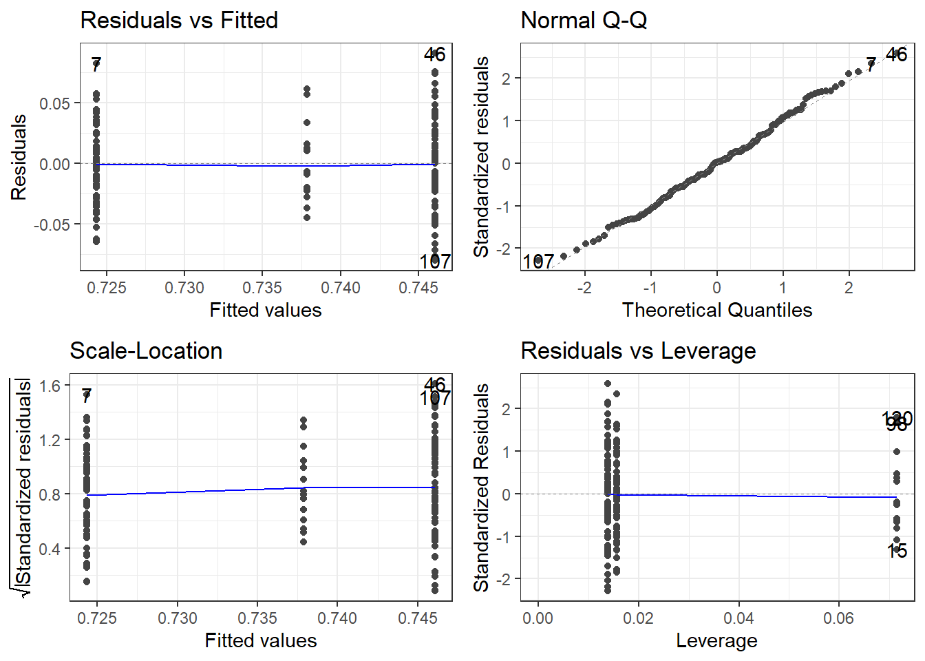

oasis %>%
  group_by(Group) %>%
  summarise(SD = sd(nWBV),
            Mean = mean(nWBV),
            n = length(nWBV))

# A tibble: 3 × 4
  Group           SD  Mean     n
  <chr>        <dbl> <dbl> <int>
1 Converted   0.0330 0.738    14
2 Demented    0.0315 0.724    64
3 Nondemented 0.0387 0.746    72

The variability looks a bit smaller in the middle group, i.e., the Converted group. HOWEVER, that is only because there are so few observations in that group.

The normality looks pretty good.

6.2.2 Testing for Constant Variability/Homoskedasticity: Levene’s Test and Brown-Forsythe Test

To test for for constant variability in ANOVA, we use ANOVA.

The hypotheses are

\(H_0: \sigma_1 = \sigma_2 = \dots = \sigma_t\) \(H_1:\) At least one difference exists.

Instead of using the observations \(y_{ij}\), we use

\[z_{ij} = |y_{ij} - \overline y_{i.}|\]

or

\[z_{ij} = |y_{ij} - \tilde y_{i.}|\]

where \(\tilde y_{i.}\) is the median of a group.

• We call it Levene’s Test when using the mean \(\overline y_{i.}\) to compute \(z_{ij}\).
• We call it the Brown-Forsythe Test when using the median \(\tilde y_{i}\) to compute \(z_{ij}\).

Then the ANOVA process is used to to see if the mean of the \(z\) values differ between the groups.

• \(SST^* = \sum^n_{i=1} n_i\left(\overline z_{i.} - \overline z_{..}\right)^2\)
• \(SSE^* = \sum^n_{i=1} \left(z_{ij} - \overline z_{i.}\right)^2\)

\(\overline z_{i.}\) and \(\overline z_{..}\) are the group means and overall mean of the \(z_{ij}\)’s.

And then we have the mean squares. Just as before.

• \(MST^* = SST/(t-1)\)
• \(MSE^* = SSE/(N-t)\)

And our test statistic is

\[F^*_t = MST^*/MSE^*\]

• Under the null hypothesis this test statistic followsan \(F(t-1, N-t)\) distribution which is used to compute its p-value.

FYI: In many texts that I have seen, it is sometimes referred to as \(W\) instead of \(F_t^*\).

6.2.3 What if the assumptions are violated?

• Should normality be a major issue, then either transformations should be attempted to try to normalize the residuals
  • Alternatively non-parametric options or GLMs could be considered.
• “Robust” standard errors could also be utilized to aid with issues regarding comparing groups (i.e., make it more robust to potential errors)

6.2.4 Some Extra Remarks

From this ResearchGate question.

Bruce Weaver writes what I consider to be some rather nice advice.

A quick summary:

1. Levene’s test is a test of homogeneity of variance, not normality.

2. Testing for normality as a precursor to a t-test or ANOVA is not a good idea. As the sample sizes increase, the sampling distribution of the mean converges on the normal distribution, and normality of the raw scores (within groups) becomes less and less important. But at the same time, the test of normality has more and more power, and so will detect unimportant departures from normality.

3. Rather than testing for normality, I would ask if it is fair and reasonable to use means and SDs for description. If it is, then ANOVA should be fairly valid.

4. Many authors likewise do not recommend testing for homogeneity of variance prior to doing a t-test or ANOVA. Box said that doing a preliminary test of variances was like putting out to sea in a row boat to see if conditions are calm enough for an ocean liner. I.e., he was saying that ANOVA is very robust to heterogeneity of variance. That is especially so when the sample sizes are equal (or nearly so). But as the sample sizes become more discrepant, heterogeneity of variance becomes very problematic. When sample sizes are reasonably similar, some authors suggest that ANOVA is robust to heterogeneity of variance so long as the ratio of largest variance to smallest variance is no more than 5:1.

However, let me add a note:

• It may not necessarily be useful to test for homogeneity of variance (and other assumptions), but it is good to inspect plots of the assumptions. If there is a huge discrepancy, then you’re going to want to address them.

6.2.4.1 One Final Note: Sample Sizes

Hopefully you end up taking a class in “Experimental Design”.

• There will be an emphasis on experiments with “balanced” data, i.e., each group has equal sample size.
• Often this will be impossible.
• Especially in experiments involving people.
• I have tried to provide tools that are robust alternatives.
  • A caveat is that if you have extremely unbalanced samples, e.g., 5 in one group and 50 in another group.
  • You should be very careful and probably need to learn new methods or consult a statistician.

6.3 Balanced (Uniform Sample Size) Two-Way ANOVA

Here are some packages for this part of the module.

# Here are the libraries I used
library(tidyverse) # standard
library(knitr) 
library(readr) 
library(ggpubr) # allows for stat_cor in ggplots
library(ggfortify) # Needed for autoplot to work on lm()
library(gridExtra) # allows me to organize the graphs in a grid
library(car) # need for some regression stuff like vif
library(GGally)
library(emmeans)

# This changes the default theme of ggplot
old.theme <- theme_get()
theme_set(theme_bw())

The idea of analysis of variance mainly stems from concepts of “experimental design” which is a separate course that should be taken should you be in a field that heavily focuses on, well… quantitative experiments that will be analyzed.

There is so much there that we can’t even touch on it in a meaningful way with the scope of this course.

Anyway, in an experiment we manipulate external variables and see their affect on the response variable.

• \(y\) is our response variable
• We can have various \(x\) variables that we are manipulating.
  • In ANOVA context these are called factors.
  • We can have more than one factor. (Technically as many as we want, but probably stop at 3!)
  • Each factor has a set of levels, i.e. the specific values that are set
  • A treatment is the specific combination of the levels of all the factors.
  • Each individual treatment could be referred to as a cell.
• Group A: A_1_,A_2_,A_3_
• Group B: B_1_, B_2_
• Group Combinations: A_1_B_1_,A_2_B_1_,A_3_B_1_,A_1_B_2_,A_2_B_2_,A_3_B_2_

6.3.1 Pseudo-Example

We are doing an ANOVA type experiment.

• We have are subjects and we want to test the effectiveness of a drug and exercise regime on blood pressure.
• The drug is factor A and there will be 3 dose levels: 0mg (control), 5mg, and 10mg
• The exercise regime is factor B with 3 levels: none (control), light, heavy.
• This would be referred to as a 3 by 3 (\(3\times3\)) ANOVA.
  • In general we say \(A\times B\) where we put the number of levels for each factor.
  • In this case there would be 9 total unique combinations of the two factors which means there would be 9 treatments

We can view it as a grid kind of pattern for the design of the experiement.

Regime\Dose	0mg	5mg	10mg
none	0 & none (control)	5 & none	10 & none
light	0 & light	5 & light	10 & light
heavy	0 & heavy	5 & heavy	10 & heavy

And there would be a random assignment of each treatment to a set of subjects.

6.3.1.1 Sample Sizes in Two-Way ANOVA

• A basic analysis is possible if there is only one subject per treatment (cell).
  • This is not an ideal scenario.
• More than 1 subject per treatment is better.
• An equal number of subjects for each treatment is “best”, which is called a balanced design
  • This may not feasible many times when involving living individuals (humans or otherwise.
  • Subject smay drop out of studies for various reasons.
  • Levels of factors may have different difficulties for obtaining/producing.
  • Variability of subject availability depending on treatments.
  • Etc.
• If there are not an equal number of individuals within each group, it is referred to as an unbalanced design.
• This usually not a problem with a large enough sample size and when there isn’t heteroscedasticity (check your assumptions!)

We will cover Balanced Design.

Unbalanced Design requires much more care and you should consult someone with experience.

Should time allow, we will cover it. But it really is just a mess to wrap your head around.

6.3.2 Notation and jargon

There’s a lot here. The notation logic is fairly procedural (to a degree that it becomes confusing).

Factors and Treatments

We have factor A with levels \(i = 1,2, \dots, a\) and factor B with levels \(j = 1,2, \dots, b\).

• \(A_i\) represents level \(i\) of factor \(A\).
• \(B_j\) represents level \(j\) of factor \(B\).
• \(A_iB_j\) represents the treatment combination of level \(i\) and level \(j\) of factors A and B respectively.
• This is sometimes referred to as “treatment ij”.

Observations and Sample Means

An individual observation is denoted by \(y_{ijk}\). The subscripts indicate we are looking at observation \(k\) from treatment \(A_iB_j\)

• There are \(n\) observations in each individual treatment treatment, \(k = 1,2, \dots, n\).
• \(\overline y_{ij.}\) is the mean of the observations in treatment \(A_iB_j\). (\(\overline y_{ij.} =\frac{1}{n} \sum_{k=1}^{n}y_{ijk}\))
• \(\overline y_{i..}\) is the mean of the observations in treatment \(A_i\) across all levels of factor B. (\(\overline y_{i..} = \frac{1}{bn}\sum_{j=1}^{b}\sum_{k=1}^{n}y_{ijk}\))
• \(\overline y_{.j.}\) is the mean of the observations in treatment \(B_j\) across all levels of factor A. (\(\overline y_{.j.} = \frac{1}{an}\sum_{i=1}^{a}\sum_{k=1}^{n}y_{ijk}\))
• \(\overline y_{...}\) is the mean of all observations. (\(\overline y_{...} = \frac{1}{abn}\sum_{i=1}^{a}\sum_{j=1}^{b}\sum_{k=1}^{n}y_{ijk}\))

6.3.3 Two way ANOVA Model

There is a means model:

\[y = \mu_{ij} + \epsilon\]

• \(\mu_{ij}\) is the mean of treatment \(A_iB_j\).
• Epsilon is the error term and it is assumed \(\epsilon \sim N(0, \sigma)\).
  • The constant variability assumption is here.

Which in my opinion is not congruent with what we are trying to investigate in Two-Way ANOVA.

• We are trying to understand the effect that both factors have on the the response variable.
• There may be an interaction between the factors.
  • This is when the effect the levels of factor A is not consistent across all levels of factor B, and vice versa.
  • For example, the mean of the response variable may increase when going from treatment \(A_1B_1\) to \(A_2B_1\), but the response variable mean decreases when we look at \(A_1B_2\) to \(A_2B_2\).

With this all in mind, the effects model in two-way ANOVA is:

\[y = \mu + \alpha_i + \beta_j + \gamma_{ij} + \epsilon\]

• \(\mu\) would be the mean of the response variable without the effects of the factors.
  • This can usually be thought of as the mean of a control group.
• \(\alpha_i\) can be thought of as the effect that level \(i\) of factor A has on the mean of \(y\).
• Likewise, \(\beta_j\) is the effect that level \(j\) of factor B has on the mean of \(y\).
• \(\gamma_{ij}\) is the interaction effect, which is the additional effect that the specific combination \(A_i\) and \(B_j\) has on the mean of \(y\).

6.3.3.1 Estimating model parameters (Means model)

If we are considering a means model there are a few things we can consider:

• The overall mean of the data \(\mu_{..}\) which is estimated by \(\overline y_{...}\)
• The overall mean of \(A_i\) (when averaged over factor B) \(\mu_{i.}\) which is estimated by \(\overline y_{i..}\)
• The overall mean of \(B_j\) (when averaged over factor B) \(\mu_{.j}\) which is estimated by \(\overline y_{.j.}\)
• The treatment mean of \(A_iB_j\) \(\mu_{ij}\) which is estimated by \(\overline y_{ij.}\)

6.3.3.2 Estimating model parameters (Effects model)

It might be more interesting to estimate how big the effect is of a given treatment or how large an interaction is.

• I would argue that the only meaningfully done IF there is a control group in both factors.

Assume that \(A_1\) and \(B_1\) are the control levels.

• Then \(\alpha_1\) and \(\beta_1\) should be (at least conceptually) \(0\).
• There would be no interaction terms for any treatment \(A_1B_j\) or \(A_iB_j\)
• \(\widehat \alpha_i = \overline y_{i..} - \overline y_{1..}\)
• \(\widehat \beta_i = \overline y_{.j.} - \overline y_{.1.}\)
• \(\widehat \gamma_{ij} = \overline y_{ij.} - \overline y_{i1.} - \overline y_{1j.} + \overline y_{ij.}\)

Estimating the interactions involves things we call contrasts and that is another can of worms.

6.3.4 Hypothesis Tests

There are three sets of hypotheses that can potentially be tested in ANOVA.

6.3.4.1 Main Effects Tests

We can test whether factor A has an effect.

\(H_0: \alpha_i = 0\) for all \(i\), i.e., factor A has no effect on the mean of \(y\).

• Note that this would be the hypothesis if there were a control group.
• Otherwise it would be more correct to say that all levels of factor A have an equivalent effect (\(\alpha_1 = \alpha_2 = \dots = \alpha_a\))

\(H_1:\) \(\alpha_i \neq 0\) for at least one \(i\). At least one level of factor A has an effect on the mean of \(y\).

• Or without a control, at least one \(\alpha_i\) differs from the rest.

Likewise we can perform a separate test for whether factor \(B\) has an effect:

\(H_0: \beta_j = 0\) for all \(j\), i.e., factor B has no effect on the mean of \(y\).

• Note that this would be the hypothesis if there were a control group.
• Otherwise it would be more correct to say that all levels of factor B have an equivalent effect (\(\beta_1 = \beta_2 = \dots = \beta_b\))

\(H_1:\) \(\beta_j \neq 0\) for at least one \(j\). At least one level of factor B has an effect on the mean of \(y\).

• Or without a control, at least one \(\beta_i\) differs from the rest.

6.3.4.2 Interaction Test

BEFORE Before you can rely on the tests for the main effects, you must first consider testing for whether there is any meaningful interaction.

\(H_0\): \(\gamma_{ij} = 0\) for all \(A_iB_j\) treatment combinations.

• The idea of changing the hypothesis for whether there is a control or not is a bit more technical.
• You could say the effects are all equivalent but then there really isn’t an interaction.
• There are multiple valid hypotheses IMO. So stick with this one to avoid getting too technical.

\(H_1: \gamma_{ij} \neq 0\) for at least on \(A_iB_j\) treatment combination.

The reason that this test must be the first one to be considered is that if there is an interaction effect, it becomes mathematically impossible to effectively conclude the strength of an effect of an individual factor overall.

• Interaction implies the effect of one factor changes depending on another factor so statements about individual factors are a moot point.

6.3.4.3 Sums of Squares, Mean Squares, and Test Statistics

We are going to ignore all the formula based stuff at this point, just consider the concepts.

• We measure how meaningful a factor or interaction is via sums of squares, just as before.
• \(SSA\) measures how meaningful is factor A within the data.
  • The degrees of freedom is \(a - 1\).
• \(SSB\) measures how meaningful is factor B within the data.
  • The degrees of freedom is \(b - 1\)
• \(SSAB\) measures how meaningful is the interaction within the data.
  • The degrees of freedom is \((a-1)(b-1)\)
• \(SSE\) is the measure of how much variability is left unexplained by the factors and interaction.
  • The degrees of freedom is \(ab(n-1)\)

“Meaningful” translates to “the amount of variability in data the data that is explained by including the variable in the model”.

Just as before, to get test statistics we need to compute mean squares.

• \(MSA = SSA/(a-1)\)
• \(MSB = SSB/(b-1)\)
• \(MSAB = SSAB/(a-1)(b-1)\)
• \(MSE = SSE/(ab(n-1))\)

And then we get \(F\) test statistics.

• \(F_A = MSA/MSE\) tests whether factor A has an effect, \(H_0: \alpha_i = 0\) for all \(i\).
• \(F_B = MSB/MSE\) tests whether factor B has an effect, \(H_0: \beta_j = 0\) for all \(j\).
• \(F_{AB} = MSAB/MSE\) tests whether there is an interaction effect, \(H_0\): \(\gamma_{ij} = 0\) for all \(i\) and \(j\).

6.3.4.4 And so there is a Two-Way ANOVA table (surprise)

Source	SS	df	MS	F	p
Factor A	\(SSA\)	\(a-1\)	\(MSA=SSA/(a-1)\)	\(F_A = MSA/MSE\)	\(p_A\)
Factor B	\(SSB\)	\(b-1\)	\(MSB=SSB/(b-1)\)	\(F_B = MSB/MSE\)	\(p_B\)
Interaction: A*B	\(SSAB\)	\((a-1)(b-1)\)	\(MSAB = SSAB/((a-1)(b-1))\)	\(F_{AB} = MSAB/MSE\)	\(p_{AB}\)
Error	\(SSE\)	\(ab(n-1)\)	\(MSE = SSE/(ab(n-1))\)

• Reject \(H_0\) if \(p < \alpha\)
• \(P_A \rightarrow H_0: \alpha_i = 0\)
• \(P_A \rightarrow H_0: \beta_j = 0\)
• \(P_{AB} \rightarrow H_0: \gamma_i = 0\)

6.3.5 Study: Compulsive Checking and Mood

This data is taken from the textbook resources of: Discovering Statistics Using R by Andy Field, Jeremy Miles, Zoë Field

which itself is using data from a journal article (one textbook author is a paper co-author):

The perseveration of checking thoughts and mood–as–input hypothesis by Davey et al. (2003), https://doi.org/10.1016/S0005-7916(03)00035-1.

The study investigated the relation between mood and when people will stop performing a task under different stopping rules. They were trying to explore the connection with Obsessive Compulsive Disorder.

• There were 60 participants (it was one of those college student studies).
• The mood of a participant was “induced” via music:
  • 20 were assigned to have a “negative” mood induction.
  • 20 were assigned to have a “positive” mood induction.
  • 20 were assigned to have a “neutral” mood induction.
• Participants were then asked to “to write down all the things they would wish to check for safety or security reasons in their home before they left for a 3-week holiday”.
• Within each mood group:
  • 10 participants were told to continue the task only if they felt like continuing.
  • 10 participants were told to continue the task until they’ve listed as many as they can.

Data are available in compulsion.csv.

• items: how many items a participant listed.
• mood: which mood induction group the participant was in.
  • Negative
  • Positive
  • Neutral
• stopRule: what was the stopping rule
  • Many : “As many as you can”
  • Feel : “Feel like continuing”

ocd <- read_csv(here::here("datasets",'ocd.csv'))

Here is what a sample of the data look like

# A tibble: 10 × 3
   items mood     stopRule
   <dbl> <chr>    <chr>   
 1    10 Neutral  Feel    
 2     7 Negative Feel    
 3    10 Positive Many    
 4     7 Neutral  Feel    
 5     5 Neutral  Many    
 6    11 Neutral  Feel    
 7     5 Neutral  Feel    
 8     5 Positive Many    
 9     8 Positive Feel    
10     9 Negative Feel    

For videos related to the analysis of this data in R, I’ll go over some issues with the analyses performed. We are basically following along with what was done in the paper.

6.3.5.1 Examining the data

Always take a look at your data first.

We’ll look at boxplots, you can group by mood and color by stopping rule.

ggplot(ocd, aes(y = items, x = mood, color = stopRule)) +
  geom_boxplot()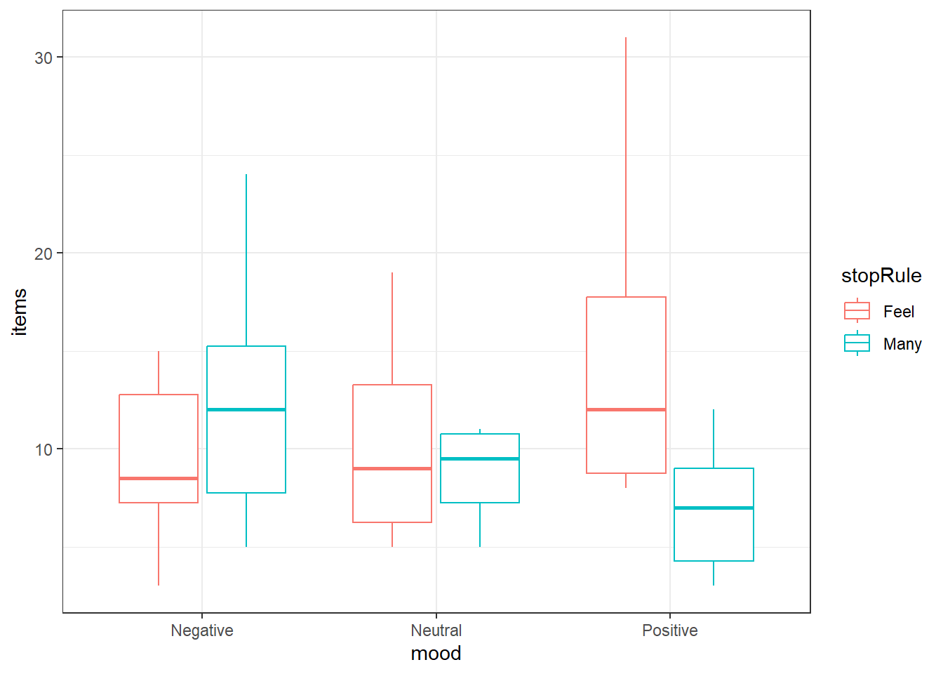

6.3.5.2 Performing two-way ANOVA

ANOVA is similar to before and we can add variables like in regression. There is a trick to adding in an interaction.

You specify the interaction of two variables by “multiplying” them with the : symbol in the formula, e.g., y ~ x + z + x:z

For two-way ANOVA, I highly recommend always using the Anova() function from the car package, not the Anova() function. The reason will be clarified

ocd.fit <- lm(items ~ mood + stopRule + mood:stopRule, 
              data = ocd)

car::Anova(ocd.fit)

Anova Table (Type II tests)

Response: items
               Sum Sq Df F value   Pr(>F)   
mood            34.13  2  0.6834 0.509222   
stopRule        52.27  1  2.0928 0.153771   
mood:stopRule  316.93  2  6.3452 0.003349 **
Residuals     1348.60 54                    
---
Signif. codes:  0 '***' 0.001 '**' 0.01 '*' 0.05 '.' 0.1 ' ' 1

Equivalently, you could “multiply” via the * symbol without listing the individual variables.

• The * tells R to include all individual AND interaction terms when used in a formula, e.g., y ~ x*z

So equivalently we could do:

ocd.fit2 <- lm(items ~ mood*stopRule, data = ocd)
Anova(ocd.fit2)

Anova Table (Type II tests)

Response: items
               Sum Sq Df F value   Pr(>F)   
mood            34.13  2  0.6834 0.509222   
stopRule        52.27  1  2.0928 0.153771   
mood:stopRule  316.93  2  6.3452 0.003349 **
Residuals     1348.60 54                    
---
Signif. codes:  0 '***' 0.001 '**' 0.01 '*' 0.05 '.' 0.1 ' ' 1

And we get equivalent results.

6.3.6 Post-hoc Comparisons: Estimated Marginal Means

Depending how we want to view the data, the means we are interested in may change.

• If we want to (and can) investigate the main effects, we look at what are referred to as the marginal means
  • \(\overline y_{i..}\) is the marginal mean of level \(i\) of factor A. (Averaged across all levels of B)
  • \(\overline y_{.j.}\) is the marginal mean of level \(j\) of factor B. (Averaged across all levels of A)
• \(\overline y_{ij.}\)’s are known as the cell or treatment means. The mean of treatment \(A_iB_j\)

6.3.6.1 Using the emmeans() function to get marginal or cell means

The emmeans() function within the eponymous emmeans package.

We will stick with the simplest way.

• The format is emmeans(model, specs, level = 0.95)
• model is the lm or other type of model you create.
• specs specifies what means you want and how you want to adjust them.
  • The input is a formula style but without the response variable listed, i.e., ~ x and not y ~ x (unless you know some more “fun” stuff).
  • ~ A will compute the marginal means for each level of factor A. This should only be used if an interaction term is not “significant”.
  • ~ A | B will calculate the cell means for the levels of factor A conditioned upon what the level of factor B is.
  • ~ A | B is a way of organizing the interaction means in a Two-Way model
  • You can switch which variable. B | A.
  • When you specify at condition variable using | you are getting only the a portion of the interaction means.
  • ~ A*B will compute the cell/interaction means
• level specifies the confidence level of resulting confidence interval
• There is an adjust argument, it is tukey by default and lets just leave it like that.
  • adjust with change automatically depending on the situation.

emmeans(ocd.fit, ~ mood, level = 0.99)

 mood     emmean   SE df lower.CL upper.CL
 Negative   10.9 1.12 54     7.92     13.9
 Neutral     9.3 1.12 54     6.32     12.3
 Positive   10.9 1.12 54     7.92     13.9

Results are averaged over the levels of: stopRule 
Confidence level used: 0.99 

emmeans(ocd.fit, ~ mood | stopRule, level = 0.99)

stopRule = Feel:
 mood     emmean   SE df lower.CL upper.CL
 Negative    9.2 1.58 54     4.98     13.4
 Neutral     9.9 1.58 54     5.68     14.1
 Positive   14.8 1.58 54    10.58     19.0

stopRule = Many:
 mood     emmean   SE df lower.CL upper.CL
 Negative   12.6 1.58 54     8.38     16.8
 Neutral     8.7 1.58 54     4.48     12.9
 Positive    7.0 1.58 54     2.78     11.2

Confidence level used: 0.99 

emmeans(ocd.fit, ~ mood:stopRule, level = 0.99)

 mood     stopRule emmean   SE df lower.CL upper.CL
 Negative Feel        9.2 1.58 54     4.98     13.4
 Neutral  Feel        9.9 1.58 54     5.68     14.1
 Positive Feel       14.8 1.58 54    10.58     19.0
 Negative Many       12.6 1.58 54     8.38     16.8
 Neutral  Many        8.7 1.58 54     4.48     12.9
 Positive Many        7.0 1.58 54     2.78     11.2

Confidence level used: 0.99 

Note that it warns you that an interaction is present and therefore you should not look at single factor means. (How convenient.)

6.3.6.2 Getting pairwise comparisons

To get pairwise comparisons, you save your emmeans() as a variable and pass it to the pairs() function.

The format is `pairs(emmeansThing, adjust = “tukey”)

• adjust will adjust resulting confidence intervals or hypothesis tests based on any of the methods discussed.
  • “tukey” is an option, use this option when doing pairwise comparisons unless you have unbalanced data
  • “sidak” is another option.
  • there are many more

moodMeans <- emmeans(ocd.fit, ~ mood, level = 0.99)
stopRuleBymoodMeans <- emmeans(ocd.fit, ~ stopRule | mood, level = 0.99)
interactionMeans <- emmeans(ocd.fit, ~ mood:stopRule, level = 0.99)

pairs(moodMeans, adjust = "tukey")

 contrast            estimate   SE df t.ratio p.value
 Negative - Neutral       1.6 1.58 54   1.012  0.5723
 Negative - Positive      0.0 1.58 54   0.000  1.0000
 Neutral - Positive      -1.6 1.58 54  -1.012  0.5723

Results are averaged over the levels of: stopRule 
P value adjustment: tukey method for comparing a family of 3 estimates 

pairs(stopRuleBymoodMeans, adjust = "tukey")

mood = Negative:
 contrast    estimate   SE df t.ratio p.value
 Feel - Many     -3.4 2.23 54  -1.521  0.1340

mood = Neutral:
 contrast    estimate   SE df t.ratio p.value
 Feel - Many      1.2 2.23 54   0.537  0.5935

mood = Positive:
 contrast    estimate   SE df t.ratio p.value
 Feel - Many      7.8 2.23 54   3.490  0.0010

pairs(interactionMeans, adjsut = "tukey")

 contrast                      estimate   SE df t.ratio p.value
 Negative Feel - Neutral Feel      -0.7 2.23 54  -0.313  0.9996
 Negative Feel - Positive Feel     -5.6 2.23 54  -2.506  0.1406
 Negative Feel - Negative Many     -3.4 2.23 54  -1.521  0.6523
 Negative Feel - Neutral Many       0.5 2.23 54   0.224  0.9999
 Negative Feel - Positive Many      2.2 2.23 54   0.984  0.9210
 Neutral Feel - Positive Feel      -4.9 2.23 54  -2.192  0.2582
 Neutral Feel - Negative Many      -2.7 2.23 54  -1.208  0.8310
 Neutral Feel - Neutral Many        1.2 2.23 54   0.537  0.9944
 Neutral Feel - Positive Many       2.9 2.23 54   1.298  0.7850
 Positive Feel - Negative Many      2.2 2.23 54   0.984  0.9210
 Positive Feel - Neutral Many       6.1 2.23 54   2.729  0.0859
 Positive Feel - Positive Many      7.8 2.23 54   3.490  0.0118
 Negative Many - Neutral Many       3.9 2.23 54   1.745  0.5090
 Negative Many - Positive Many      5.6 2.23 54   2.506  0.1406
 Neutral Many - Positive Many       1.7 2.23 54   0.761  0.9729

P value adjustment: tukey method for comparing a family of 6 estimates 

Note the p-values are adjusted depending on how many groups are being compared:

mood = Positive:
 contrast                                  estimate   SE df t.ratio p.value
 As many as you can - Feel like continuing     -7.8 2.23 54 -3.490  0.0010 

Differs from:

 contrast                      estimate   SE df t.ratio p.value p.value
 Positive Feel - Positive Many      7.8 2.23 54  3.490  0.0118  

6.3.7 Diagnostics

Residual diagnostics are just like before. Use the autoplot() function to gauge how the assumptions are holding.

autoplot(ocd.fit)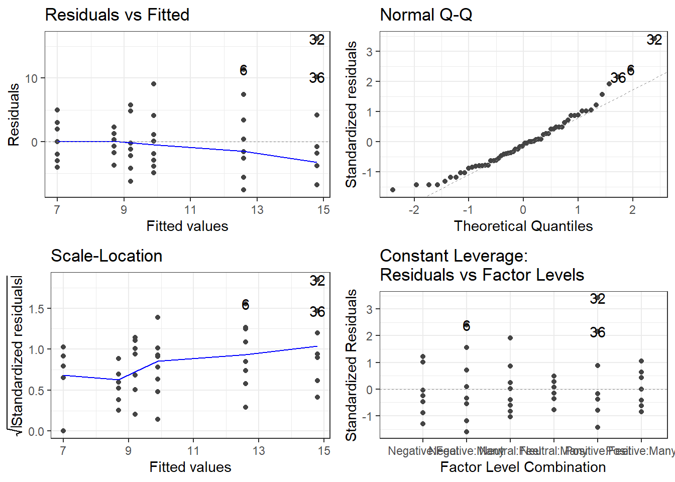

And if you feel as if you need it, use the leveneTest() function in the car package to get the Brown-Forsythe test (because levene’s apparently isn’t the default!)

This must be done at the cell means level, and leveneTest doesn’t play nice with Two-Way ANOVA models. You have to specify a formula with JUST the interaction term.

leveneTest(items ~ mood:stopRule, ocd)

Levene's Test for Homogeneity of Variance (center = median)
      Df F value Pr(>F)
group  5  1.7291 0.1436
      54               

6.4 Unbalanced Two-Factor Analysis of Variance

Here are some code chunks that setup this chapter.

# This sets the default behavior for R chunks when knitted.
# echo = TRUE, by default code is displayed
# message and warning = FALSE prevent extra stuff 
# being in the knitted document.
# When you run the code chunk while inside the Rmd file, 
# you will still see
# warnings and messages
knitr::opts_chunk$set(echo = TRUE, message = FALSE, warning = FALSE)

# Here are the libraries I used
library(tidyverse) # standard
library(knitr) 

library(readr) # need to read in data
library(ggpubr) # allows for stat_cor in ggplots
library(ggfortify) # Needed for autoplot to work on lm()
library(gridExtra) # allows me to organize the graphs in a grid
library(car) # need for some regression stuff like vif
library(GGally)
library(emmeans)

# This changes the default theme of ggplot
old.theme <- theme_get()
theme_set(theme_bw())

An Unbalanced ANOVA involves data where individual treatments/cells do not have the same number of observations/subjects.

The principals remain the same:

• \(y\) is our response variable
• We can have various \(x\) variables that we are manipulating.
  • In ANOVA context these are called factors.
  • We can have more than one factor. (Technically as many as we want, but probably stop at 3!)
  • Each factor has a set of levels, i.e. the specific values that are set
  • A treatment is the specific combination of the levels of all the factors.
• We wish to assess which factors are important in our response variable.
• The main diffference with unbalanced data is that the hypothesis tests become a little more obtuse.

6.4.1 Two way ANOVA Model

This is still the same! It’s just copy pasted from previous section.

There is a means model:

\[y = \mu_{ij} + \epsilon\]

• \(\mu_{ij}\) is the mean of treatment \(A_iB_j\).
• Epsilon is the error term and it is assumed \(\epsilon \sim N(0, \sigma)\).
  • The constant variability assumption is here.

Which in my opinion is not congruent with what we are trying to investigate in Two-Way ANOVA.

• We are trying to understand the effect that both factors have on the the response variable.
• There may be an interaction between the factors.
  • This is when the effect the levels of factor A is not consistent across all levels of factor B, and vice versa.
  • For example, the mean of the response variable may increase when going from treatment \(A_1B_1\) to \(A_2B_1\), but the response variable mean decreases when we look at \(A_1B_2\) to \(A_2B_2\).

With this all in mind, the effects model in two-way ANOVA is:

\[y = \mu + \alpha_i + \beta_j + \gamma_{ij} + \epsilon\]

• \(\mu\) would be the mean of the response variable without the effects of the factors.
  • This can usually be thought of as the mean of a control group.
• \(\alpha_i\) can be thought of as the effect that level \(i\) of factor A has on the mean of \(y\).
• Likewise, \(\beta_j\) is the effect that level \(j\) of factor B has on the mean of \(y\).
• \(\gamma_{ij}\) is the interaction effect, which is the additional effect that the specific combination \(A_i\) and \(B_j\) has on the mean of \(y\).

6.4.2 Notation and jargon

There’s a lot here. The notation logic is fairly procedural (to a degree that it becomes confusing).

Factors and Treatments

We have factor A with levels \(i = 1,2, \dots, a\) and factor B with levels \(j = 1,2, \dots, b\).

• \(A_i\) represents level \(i\) of factor \(A\).
• \(B_j\) represents level \(j\) of factor \(B\).
• \(A_iB_j\) represents the treatment combination of level \(i\) and level \(j\) of factors A and B respectively.
• This is sometimes referred to as “treatment ij”.

Sample Sizes

This is where things get sketchier/more obsuse. We have to account for the fact that each \(A_iB_j\) treatment group may have a different sample size.

• \(n_{ij}\) is the number of observations/subjects in treatment \(A_iB_j\).
• \(n_{i.}\) represents the total number of observations in \(A_i\). (\(n_{i.} = \sum_{j=1}^bn_{ij}\))
• \(n_{.j}\) represents the total number of observations in level \(i\) of factor A. (\(n_{.j} = \sum_{i=1}^a n_{ij}\))
• \(n_{..}\) (or sometimes \(N\)) represents the total number of observations overall. (\(n_{..} = \sum_{i=1}^a \sum_{j=1}^b n_{ij}\))

Observations and Sample Means

An individual observation is denoted by \(y_{ijk}\). The subscripts indicate we are looking at observation \(k\) from treatment \(A_iB_j\)

• Since there are \(n_{ij}\) observations in each individual treatment treatment, \(k = 1,2, \dots, n_{ij}\).
• \(\overline y_{ij.}\) is the mean of the observations in treatment \(A_iB_j\). (\(\overline y_{ij.} =\frac{1}{n_{ij}} \sum_{k=1}^{n_{ij}}y_{ijk}\))
• \(\overline y_{i..}\) is the mean of the observations in treatment \(A_i\) across all levels of factor B. (\(\overline y_{i..} = \frac{1}{n_{i.}}\sum_{j=1}^{b}\sum_{k=1}^{n_{ij}}y_{ijk}\))
• \(\overline y_{.j.}\) is the mean of the observations in treatment \(B_j\) across all levels of factor A. (\(\overline y_{.j.} = \frac{1}{n_{.j}}\sum_{i=1}^{a}\sum_{k=1}^{n_{ij}}y_{ijk}\))
• \(\overline y_{...}\) is the mean of all observations. (\(\overline y_{...} = \frac{1}{n_{..}}\sum_{i=1}^{a}\sum_{j=1}^{b}\sum_{k=1}^{n_{ij}}y_{ijk}\))

6.4.3 Sums of Squares in Unbalanced Designs

This is where things get tricky in unbalanced designs. We are forgoing formulas at this point because they become somewhat less meaningful.

• In order for you to safely perform these hypothesis tests, you have to consider how you are testing them.
• If we were to follow the pattern of say multiple regression or one-way ANOVA, we could separate the variability explained by each factor.

\[SSA = \text{Variability Explained by Factor A}\]

• SSA would what is used to test \(H_0: \alpha_i = 0\) for all \(i\).

\[SSB = \text{Variability Explained by Factor B}\]

• SSB would what is used to test \(H_0: \beta_j = 0\) for all \(j\).

\[SSAB = \text{Variability Explained by interaction between A and B}\]

• SSAB would what is used to test \(H_0: \gamma_{ij} = 0\) for all \(i,j\).

However… In unbalanced designs, we no longer have access to these simplified sums of squares and hypothesis tests

There become 3 different mainstream types of ANOVA Hypothesis Tests

6.4.4 The Forsest of Sums of Squares

There are many ways of framing the sums of squares in unbalanced ANOVA as care must be taken.

The notation here is changing to emphasize that we are looking at fundamentally different things now.

• \(SS(A)\) is the amount of variability explained by factor A in a model by itself,

• \(SS(B)\) is the amount of variability explained for by factor B in a model by itself.

• \(SS(AB)\) is the amount of variability explained for by interaction in a model by itself.

• \(SS(A|B)\) is the additional variability explained for by factor A when factor B is in the model

  • \(SS(A|B,AB)\) is the additional variability explained for by factor A when factor B and the interaction are in the model.

• \(SS(B|A)\) is the additional variability explained for by factor B when factor A is in the model.

  • \(SS(B|A,AB)\) is the additional variability explained for by factor A when factor B and the interaction are in the model.

• \(SS(AB|A,B)\) is the additional variability explained for by the interaction when factor B and A are in the model.

The sum of squares are now about how much more a factor or interaction can contribute to a model. Not whether it is in the model or not.

6.4.5 Hypothesis Tests

There are three types of tests that use these sums of squares.

• Type I: “Sequential”.
• TYpe II: “Marginality” (This is a hill some people choose to die on it seems.)
• Type III: “???”

6.4.5.1 Type I Tests

Type I tests are about sequentially adding terms, starting with the factors then moving up to higher order terms (interaction).

The sequence of hypothesis tests would be the following.

1. Start with one factor, the test would be:

• \(H_0: \mu_{ij} = \mu\)
• \(H_1: \mu_{ij} = \mu + \alpha_i\)
• This would be performed using \(SS(A)\)

2. Add in the next factor, the test would be:

• \(H_0: \mu_{ij} = \mu + \alpha_i\)
• \(H_1: \mu_{ij} = \mu + \alpha_i + \beta_j\)
• This would be performed using \(SS(B|A)\)

3. Add in the interaction.

• \(H_0: \mu_{ij} = \mu + \alpha_i + \beta_j\)
• \(H_1: \mu_{ij} = \mu + \alpha_i + \beta_j +\gamma_{ij}\)
• This would be performed using \(SS(AB|A,B)\)

6.4.5.2 Type II Tests

Type II Tests run on the principal of “marginality”.

• The idea is to move from lower order models, to higher order models with interactions.
• This becomes more important with three or more factors.

1. Compare how well factor A improves a model with factor B in it.

• \(H_0: \mu_{ij} = \mu + \beta_j\)
• \(H_1: \mu_{ij} = \mu + \alpha_i + \beta_j\)
• This would be performed using \(SS(A)\)

2. Compare how well factor B improves a model with factor A in it.

• \(H_0: \mu_{ij} = \mu + \alpha_i\)
• \(H_1: \mu_{ij} = \mu + \alpha_i + \beta_j\)
• This would be performed using \(SS(B|A)\)

3. Finally, see how well adding in the interaction works when both main effects are in the model:

• \(H_0: \mu_{ij} = \mu + \alpha_i + \beta_j\)
• \(H_1: \mu_{ij} = \mu + \alpha_i + \beta_j +\gamma_{ij}\)
• This would be performed using \(SS(AB|A,B)\)

6.4.5.3 Type III Tests

Type III tests are a kind of catch all test the compares a full model (all terms including interaction) to a model missing a single term.

1. Compare how well factor A improves a model with factor B and the interaction in it.

• \(H_0: \mu_{ij} = \mu + \beta_j +\gamma_{ij}\)
• \(H_1: \mu_{ij} = \mu + \alpha_i + \beta_j +\gamma_{ij}\)
• This would be performed using \(SS(A|B,AB)\)

2. Compare how well factor B improves a model with factor A and the interaction in it.

• \(H_0: \mu_{ij} = \mu + \alpha_i + \gamma_{ij}\)
• \(H_1: \mu_{ij} = \mu + \alpha_i + \beta_j +\gamma_{ij}\)
• This would be performed using \(SS(B|A,AB)\)

3. Finally, see how well adding in the interaction works when both main effects are in the model:

• \(H_0: \mu_{ij} = \mu + \alpha_i + \beta_j\)
• \(H_1: \mu_{ij} = \mu + \alpha_i + \beta_j +\gamma_{ij}\)
• This would be performed using \(SS(AB|A,B)\)

6.4.5.4 Which tests to use?

In simple terms, it is situationally dependent which hypothesis test you use.

In more practical terms, pretty much Type II and Type III only

• Type I should only be done if you have pre-determined the list of importance of variables, for some reason or another.
• Type II involves a more elegant approach that only becomes important in a three-way ANOVA (3 factors)
  • The general idea is that if a factor is “insignificant” then higher order terms (interactions) would/should not be in the model.
  • Type II sums of squares are most powerful for detecting main effects when interactions are not present.
• Type III is just brute force your way through the hypothesis tests.
• I see Type II recommended more often than Type III. Go ahead and use it by default, I’d say.
• But if you do not really know what is going on Type III is “safe”, in my opinion.
  • Others would argue otherwise simply by fact that another option exists and the whole “my opinion is better” mindset.
  • I personally don’t see a problem with Type III but it’s situation dependent.
  • If there are interactions, then it doesn’t even matter because you can’t ignore lower order terms anyway.
  • This guy has a VERY strong opinion on not using Type III: Page 12 of https://www.stats.ox.ac.uk/pub/MASS3/Exegeses.pdf.

6.4.5.5 PAY ATTENTION TO WHAT THE SOFTWARE DOES

 

• In unmodified/base R, an ANOVA analysis will use Type I Tests which is almost NEVER recommended.
• The Anova() function in the car package uses Type II by defaul, which is fine.
• If you want Type III sum of squares, you have to change an option in R, then use the Anova() function.
• Other software use different Type tests by default. Read the manual.

6.4.6 Patient Satisifcation Data

This data is taken from the text: Applied Regression Analysis and Other Multivariable Methods

ISBN: 9781285051086

by David G. Kleinbaum, Lawrence L. Kupper, Azhar Nizam, Eli S. Rosenberg 5th Edition | Copyright 2014

It’s a good book, but it may dive a bit too much in to theory sometimes. I don’t feel like I am shamelessly ripping from the book since they took the data from a study/dissertation:

Thompson, S.J. 1972. “The Doctor–Patient Relationship and Outcomes of Pregnancy.” Ph.D. disser-tation, Department of Epidemiology, University of North Carolina, Chapel Hill, N.C.

The study attempted to ascertain a patients satisfaction with level of medical care during pregnancy, and its association with how worried the patient was and how affective patient-doctor communication was rated.

Data are available in patSas.csv.

• Satisfaction is the patient’s self rated satisfaction with their medical care.
  • The scale is 1 through 10.
  • It is unknown whether lower is better.
  • It could be a Very Satisfied to Very Dissatisfied from left to right which would mean 1 = Very Satisfied.
• Worry is how worried a patient was.
  • Worry was grouped into the levels Negative and Postive.
  • I cannot ascertain whether Negative means they had low worry or they a negative feelings. The book source does not specify, and the dissertation is not open access.
• AffCom is the rating of how affective the patient-doctor communication was rated.
  • The levels are High, Medium, to Low.
  • It may seem more obvious what the meaning is here, but always be careful. PhD students can be quirky and have their own unique concepts of perceived reality.

6.4.6.1 Looking at the sample sizes for the cells

patSas <- read_csv(here::here(
  "datasets",'patSas.csv'))

Here is what a sample of the data look like

# A tibble: 10 × 3
   Satisfaction Worry    AffCom
          <dbl> <chr>    <chr> 
 1            5 Positive Low   
 2            6 Positive Low   
 3            6 Negative Medium
 4            3 Negative High  
 5            8 Negative Low   
 6            6 Negative High  
 7            7 Positive Low   
 8            8 Negative Low   
 9            8 Negative Low   
10            6 Positive High  

Lets look at how many patients fall into each factor level and treatment.

# Worriers breakdown
table(patSas$Worry)

Negative Positive 
      22       30 

# Communication breakdown
table(patSas$AffCom)

  High    Low Medium 
    22     18     12 

# Two-way Table
table(patSas$Worry, patSas$AffCom)

          
           High Low Medium
  Negative    8  10      4
  Positive   14   8      8

The setup is unbalanced.

• The main issue I have is the sample size in the Negative/Medium treatment cell is low compared to the others.
• If the ratio between smaller and larger groups gets too large, ANOVA starts becoming kind of pointless.
• a 4 to 14 is not terrible but definitely it is starting to get to the point where ANOVA may not be very useful.

6.4.6.2 Graphing the data! (DO IT!)

ggplot(patSas, aes(y = Satisfaction, 
                   x = AffCom, color = Worry)) +
  geom_boxplot()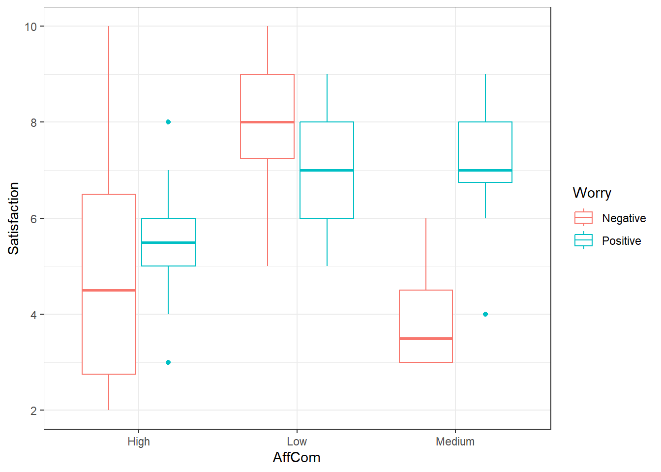

Looks like an interaction. The pattern is different in the negative group versus the positive group.

6.4.6.3 Type II ANOVA

First, lets use the default of the Anova() function in the car package.

This will do Type II Tests by default

# Make your model
pat.fit <- lm(Satisfaction ~ AffCom*Worry, patSas)

Anova(pat.fit)

Anova Table (Type II tests)

Response: Satisfaction
              Sum Sq Df F value    Pr(>F)    
AffCom        51.829  2  8.3112 0.0008292 ***
Worry          3.425  1  1.0984 0.3000824    
AffCom:Worry  26.682  2  4.2787 0.0197611 *  
Residuals    143.429 46                      
---
Signif. codes:  0 '***' 0.001 '**' 0.01 '*' 0.05 '.' 0.1 ' ' 1

Here we have somewhat strong evidence that there is an interaction.

• This wouldn’t fall under my default criteria for declaring “significance” if I were in the NHST frame of reference.
• Interaction is fairly apparent from the graphs.
• I would err on the side of caution, and declare that there is one.
  • We would have to ignore main effects, but if there is actually an interaction, main effect analyses would be difficult to interpret.
  • It might be prudent for higher \(\alpha\) values for interaction tests in general.

6.4.6.4 Type III ANOVA

To do type III ANOVA in R, specifically within the Anova() function, you have to do a couple things.

• There is a type argument so you would use Anova(model, type = "III") or type = 3.
• You need also need to specify a special option.
• Then you have to create a new model AFTER you use that option.
• This is usually the default method in most statistical software (other than car in R)

options(contrasts = c("contr.sum","contr.poly"))

pat.fit2 <- lm(Satisfaction ~ AffCom*Worry, patSas)

Anova(pat.fit2, type = 3)

Anova Table (Type III tests)

Response: Satisfaction
              Sum Sq Df  F value    Pr(>F)    
(Intercept)  1679.33  1 538.5911 < 2.2e-16 ***
AffCom         52.11  2   8.3566  0.000802 ***
Worry           8.30  1   2.6627  0.109554    
AffCom:Worry   26.68  2   4.2787  0.019761 *  
Residuals     143.43 46                       
---
Signif. codes:  0 '***' 0.001 '**' 0.01 '*' 0.05 '.' 0.1 ' ' 1

Notice that intercept term there, ignore it. That’s just telling us there is an overall mean that is not zero, which is a pointless piece of information given the scores start at 1.

6.4.6.5 Multiple Comparisons

Everything is the same as previously when using emmeans() and pairs().

• If there is an interaction, then you must use emmeans(model, ~ A:B) or A*B.
• When using pairs it is safer to use the adjust = "holm" argument.
  • Tukey procedures get more unreliable in the case of unbalanced data.
  • This procedure conserves FWER under arbitrary conditions and is better than Bonferroni.

6.4.6.6 Main Effect Comparisons

If we consider the evidence of interaction to be sufficient to conclude that there is in fact an interaction, it is arguably useless to look at main effects.

• Furthermore, we would not look at the Worry main effect means and pairwise comparisons.
• This is just for demonstration.

worryMeans <- emmeans(pat.fit, ~ Worry)

worryMeans

 Worry    emmean    SE df lower.CL upper.CL
 Negative   5.67 0.406 46     4.85     6.48
 Positive   6.52 0.334 46     5.85     7.20

Results are averaged over the levels of: AffCom 
Confidence level used: 0.95 

pairs(worryMeans)

 contrast            estimate    SE df t.ratio p.value
 Negative - Positive   -0.857 0.525 46  -1.632  0.1096

Results are averaged over the levels of: AffCom 

• There still was an interaction so this comparison may not be considered worthwhile.

comMeans <- emmeans(pat.fit, ~ AffCom)

comMeans

 AffCom emmean    SE df lower.CL upper.CL
 High     5.29 0.391 46     4.50     6.07
 Low      7.50 0.419 46     6.66     8.34
 Medium   5.50 0.541 46     4.41     6.59

Results are averaged over the levels of: Worry 
Confidence level used: 0.95 

pairs(comMeans, adjust = "holm")

 contrast      estimate    SE df t.ratio p.value
 High - Low      -2.214 0.573 46  -3.863  0.0010
 High - Medium   -0.214 0.667 46  -0.321  0.7496
 Low - Medium     2.000 0.684 46   2.924  0.0107

Results are averaged over the levels of: Worry 
P value adjustment: holm method for 3 tests 

This indicates that high and medium affective communication were associated with lower patient satisfaction scores.

6.4.6.7 One Way to Look at Interactions: AffCom by Worry Levels

We may only be interested in how affective communication affects satisfaction when looking at the individual levels of worry.

• This is a comparison of cell/interaction means.
• However, we are subsetting the comparisons we care about.

comByWorryMeans <- emmeans(pat.fit, ~ AffCom | Worry)

comByWorryMeans

Worry = Negative:
 AffCom emmean    SE df lower.CL upper.CL
 High     5.00 0.624 46     3.74     6.26
 Low      8.00 0.558 46     6.88     9.12
 Medium   4.00 0.883 46     2.22     5.78

Worry = Positive:
 AffCom emmean    SE df lower.CL upper.CL
 High     5.57 0.472 46     4.62     6.52
 Low      7.00 0.624 46     5.74     8.26
 Medium   7.00 0.624 46     5.74     8.26

Confidence level used: 0.95 

pairs(comByWorryMeans, adjust = "holm")

Worry = Negative:
 contrast      estimate    SE df t.ratio p.value
 High - Low       -3.00 0.838 46  -3.582  0.0016
 High - Medium     1.00 1.080 46   0.925  0.3599
 Low - Medium      4.00 1.040 46   3.829  0.0012

Worry = Positive:
 contrast      estimate    SE df t.ratio p.value
 High - Low       -1.43 0.783 46  -1.825  0.2233
 High - Medium    -1.43 0.783 46  -1.825  0.2233
 Low - Medium      0.00 0.883 46   0.000  1.0000

P value adjustment: holm method for 3 tests 

• So it seems that the discrepancy arises when worry levels are categorized as “Negative”
• However, even though there is low significance, the same pattern arises in the Worry = Positive group.

6.4.6.8 Or Maybe: Worry by AffCom Levels

We may only be interested in how affective communication affects satisfaction when looking at the individual levels of worry.

• This is a comparison of cell/interaction means.
• However, we are subsetting the comparisons we care about.

worryByComMeans <- emmeans(pat.fit, ~ Worry | AffCom)

worryByComMeans

AffCom = High:
 Worry    emmean    SE df lower.CL upper.CL
 Negative   5.00 0.624 46     3.74     6.26
 Positive   5.57 0.472 46     4.62     6.52

AffCom = Low:
 Worry    emmean    SE df lower.CL upper.CL
 Negative   8.00 0.558 46     6.88     9.12
 Positive   7.00 0.624 46     5.74     8.26

AffCom = Medium:
 Worry    emmean    SE df lower.CL upper.CL
 Negative   4.00 0.883 46     2.22     5.78
 Positive   7.00 0.624 46     5.74     8.26

Confidence level used: 0.95 

pairs(worryByComMeans, adjust = "holm")

AffCom = High:
 contrast            estimate    SE df t.ratio p.value
 Negative - Positive   -0.571 0.783 46  -0.730  0.4690

AffCom = Low:
 contrast            estimate    SE df t.ratio p.value
 Negative - Positive    1.000 0.838 46   1.194  0.2386

AffCom = Medium:
 contrast            estimate    SE df t.ratio p.value
 Negative - Positive   -3.000 1.080 46  -2.774  0.0080

6.4.6.9 Another way: All Pairwise Comparison (Throw everything at the wall and see what sticks)

cellMeans <- emmeans(pat.fit, ~ AffCom:Worry)

cellMeans

 AffCom Worry    emmean    SE df lower.CL upper.CL
 High   Negative   5.00 0.624 46     3.74     6.26
 Low    Negative   8.00 0.558 46     6.88     9.12
 Medium Negative   4.00 0.883 46     2.22     5.78
 High   Positive   5.57 0.472 46     4.62     6.52
 Low    Positive   7.00 0.624 46     5.74     8.26
 Medium Positive   7.00 0.624 46     5.74     8.26

Confidence level used: 0.95 

pairs(cellMeans, adjust = "holm")

 contrast                          estimate    SE df t.ratio p.value
 High Negative - Low Negative        -3.000 0.838 46  -3.582  0.0115
 High Negative - Medium Negative      1.000 1.080 46   0.925  1.0000
 High Negative - High Positive       -0.571 0.783 46  -0.730  1.0000
 High Negative - Low Positive        -2.000 0.883 46  -2.265  0.2825
 High Negative - Medium Positive     -2.000 0.883 46  -2.265  0.2825
 Low Negative - Medium Negative       4.000 1.040 46   3.829  0.0058
 Low Negative - High Positive         2.429 0.731 46   3.322  0.0229
 Low Negative - Low Positive          1.000 0.838 46   1.194  1.0000
 Low Negative - Medium Positive       1.000 0.838 46   1.194  1.0000
 Medium Negative - High Positive     -1.571 1.000 46  -1.570  0.7400
 Medium Negative - Low Positive      -3.000 1.080 46  -2.774  0.0956
 Medium Negative - Medium Positive   -3.000 1.080 46  -2.774  0.0956
 High Positive - Low Positive        -1.429 0.783 46  -1.825  0.5955
 High Positive - Medium Positive     -1.429 0.783 46  -1.825  0.5955
 Low Positive - Medium Positive       0.000 0.883 46   0.000  1.0000

P value adjustment: holm method for 15 tests 

And then you have this mess to summarize. (Cell references are in AffCom:Worry format)

• Low:Negative have higher mean scores than High:Negative, High:Positive, and Medium:Negative. (p \(\leq\) 0.0229)
• All other comparisons are inconclusive.

A generalization of this is that Low affective communication and Negative worry were associated with higher satisfaction scores.

• Hopefully this means that the scale goes from very satisfied to very dissatisfied in terms of 1 through 10 and affective communication leads to better satisfaction.
• Otherwise if a patient is categorized and “negative” on the worry skill, we should send in a doctor that sucks at communicating, apparently.

6.5 Analysis of Covariance

6.5.1 Introduction to ANCOVA

Analysis of Covariance (ANCOVA) is a statistical technique that combines features of both ANOVA (Analysis of Variance) and regression analysis. It allows researchers to:

• Compare group means while controlling for the effects of one or more continuous variables (covariates)
• Reduce error variance and increase statistical power
• Remove the influence of confounding variables

6.5.1.1 Key Components

Dependent Variable (Y): The outcome variable being measured (continuous)

Independent Variable/Factor: The categorical grouping variable (e.g., treatment groups)

Covariate(s): Continuous variable(s) that may influence the dependent variable but are not the primary focus of the study

6.5.1.2 When to Use ANCOVA

ANCOVA is particularly useful when:

1. Controlling for baseline differences: When groups differ on important variables before treatment
2. Increasing precision: When you want to reduce error variance to detect treatment effects more easily
3. Accounting for confounding variables: When continuous variables might influence your outcome
4. Pre-post designs: When you have baseline measurements and want to control for initial differences

6.5.1.3 Common Examples

• Educational Research: Comparing teaching methods while controlling for students’ prior knowledge
• Medical Studies: Comparing treatments while controlling for age, baseline severity, or other patient characteristics
• Psychology: Comparing therapy effectiveness while controlling for initial depression scores

---

6.5.1.4 ANCOVA vs. Other Analyses

Analysis	Purpose	Variables
t-test	Compare 2 group means	1 categorical IV, 1 continuous DV
ANOVA	Compare 2+ group means	1+ categorical IV, 1 continuous DV
Regression	Predict outcomes	Continuous IV(s), 1 continuous DV
ANCOVA	Compare groups while controlling for covariates	Categorical IV(s) + continuous covariate(s), 1 continuous DV

---

6.5.1.5 Key Assumptions of ANCOVA

1. Normality

• The dependent variable should be approximately normally distributed within each group
• Can be assessed using histograms, Q-Q plots, or statistical tests (Shapiro-Wilk)

2. Homogeneity of Variance

• Equal variances across groups (homoscedasticity)
• Tested using Levene’s test or by examining residual plots

3. Independence of Observations

• Each observation should be independent of others
• Addressed through proper study design and random sampling

4. Linear Relationship

• Linear relationship between the covariate and dependent variable within each group
• Assessed through scatterplots

5. Homogeneity of Regression Slopes

• Critical assumption unique to ANCOVA
• The relationship between covariate and DV should be the same across all groups
• No significant interaction between covariate and grouping variable

6. Covariate Measured Without Error

• Covariates should be reliable measures
• Measurement error in covariates can bias results

6.5.1.6 The ANCOVA Model

6.5.1.6.1 Mathematical Representation

For a one-way ANCOVA with one covariate:

\(Y_{ij} = \mu + \alpha_i + \beta(X_{ij} - \bar{X}) + \varepsilon_{ij}\)

Where:

• \(Y_{ij}\) = observed score for individual j in group i
• \(\mu\) = overall mean
• \(\alpha_i\) = effect of group i
• \(\beta\) = regression coefficient for the covariate
• \(X_{ij}\) = covariate score for individual j in group i
• \(\bar{X}\) = overall mean of the covariate
• \(\varepsilon_{ij}\) = error term

What ANCOVA Does

1. Adjusts group means based on covariate values
2. Creates “adjusted means” that represent what group means would be if all groups had the same covariate value (usually at the average; MEM)
3. Tests for significant differences between these adjusted means

6.5.1.7 Interpreting ANCOVA Results

6.5.1.7.1 Main Components of Output

Tests of Between-Subjects Effects:

• Covariate effect: Is the covariate significantly related to the DV?

• Group effect: Are there significant differences between groups after controlling for the covariate?

Adjusted Means:

• Group means after controlling for the covariate
• These are the means that would be expected if all groups had the same covariate value

6.5.1.8 Advantages and Limitations

6.5.1.8.1 Advantages

• Increased statistical power by reducing error variance
• Controls for confounding variables that might otherwise bias results
• More precise estimates of treatment effects
• Can handle pre-existing group differences

6.5.1.8.2 Limitations

• Assumes linear relationships between covariates and DV
• Requires homogeneity of regression slopes
• Cannot control for unmeasured confounds
• Covariate should not be affected by the treatment (in experimental designs)

6.5.1.9 Common Mistakes and Considerations

6.5.1.9.1 What NOT to Do

1. Don’t use post-treatment measures as covariates in experimental designs
2. Don’t ignore the homogeneity of slopes assumption
3. Don’t use highly correlated covariates (multicollinearity issues)
4. Don’t assume ANCOVA fixes all design problems

6.5.1.9.2 Best Practices

• Always check assumptions before interpreting results
• Use scatterplots to examine covariate-DV relationships
• Consider the theoretical justification for including covariates
• Report both adjusted and unadjusted means when possible

Key Takeaways

• ANCOVA combines ANOVA and regression to control for continuous variables
• It increases statistical power by reducing error variance
• The homogeneity of regression slopes assumption is critical and unique to ANCOVA
• Adjusted means represent group differences after controlling for covariates
• Proper assumption checking is essential for valid interpretation

6.5.2 Introduction to ANCOVA Assumptions

Analysis of Covariance (ANCOVA) combines ANOVA and regression by including both categorical predictors (factors) and continuous predictors (covariates). However, ANCOVA relies on several key assumptions, with homogeneity of slopes being one of the most critical.

Key ANCOVA Assumptions

1. Independence of observations
2. Normality of residuals
3. Homogeneity of variance (homoscedasticity)
4. Linearity between covariate and dependent variable
5. Homogeneity of slopes (parallel regression lines)

Today we focus on testing the homogeneity of slopes assumption.

6.5.2.1 The Homogeneity of Slopes Assumption

The homogeneity of slopes assumption requires that the relationship between the covariate and dependent variable is the same across all Groups. In other words, the regression lines for each Group should be parallel.

Why is this important?

• If slopes differ significantly between Groups, the covariate effect varies by Group
• This violates the assumption that we can “adjust” for the covariate uniformly
• Violation suggests an interaction between the factor and covariate

6.5.2.2 Setting up the Analysis in R

# Load required packages
library(tidyverse)
library(car)        # For Anova() function
library(emmeans)    # For adjusted means
library(modelbased) # For Johnson-Neyman
library(marginaleffects) # For average marginal effects
library(broom)      # For tidy model outputs
library(patchwork)  # For combining plots
library(see)
library(performance)

6.5.2.3 Simulating Example Data

Let’s create a dataset to demonstrate these concepts:

set.seed(123)
n_per_Group <- 30
Groups <- c("Control", "Treatment_A", "Treatment_B")

# Create data with different slopes for demonstration
data <- tibble(
  Group = rep(Groups, each = n_per_Group),
  covariate = rnorm(n_per_Group * 3, mean = 50, sd = 10)
) %>%
  mutate(
    # Different slopes for each Group to show violation
    outcome = case_when(
      Group == "Control" ~ 20 + 0.5 * covariate + rnorm(n(), 0, 5),
      Group == "Treatment_A" ~ 25 + 0.8 * covariate + rnorm(n(), 0, 5),
      Group == "Treatment_B" ~ 15 + 0.2 * covariate + rnorm(n(), 0, 5)
    ),
    Group = factor(Group)
  )

# Display first few rows
head(data)

# A tibble: 6 × 3
  Group   covariate outcome
  <fct>       <dbl>   <dbl>
1 Control      44.4    47.2
2 Control      47.7    46.6
3 Control      65.6    54.0
4 Control      50.7    42.2
5 Control      51.3    52.4
6 Control      67.2    50.6

6.5.2.4 Visual Assessment of Homogeneity of Slopes

6.5.2.4.1 Method 1: Scatterplot with Separate Regression Lines

p1 <- ggplot(data, aes(x = covariate, y = outcome, color = Group)) +
  geom_point(alpha = 0.6) +
  geom_smooth(method = "lm", se = TRUE) +
  labs(
    title = "Visual Assessment: Separate Regression Lines",
    subtitle = "Non-parallel lines suggest violation of homogeneity of slopes",
    x = "Covariate",
    y = "Outcome Variable",
    color = "Group"
  ) +
  scale_color_brewer(type = "qual", palette = "Set1")

print(p1)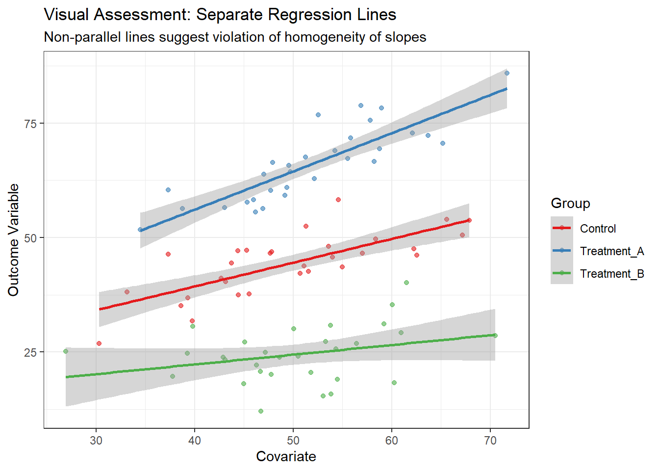

6.5.2.4.2 Method 2: Faceted Plots

p2 <- ggplot(data, aes(x = covariate, y = outcome)) +
  geom_point(alpha = 0.6) +
  geom_smooth(method = "lm", se = TRUE, color = "blue") +
  facet_wrap(~Group) +
  labs(
    title = "Visual Assessment: Faceted by Group",
    subtitle = "Compare slopes across panels",
    x = "Covariate",
    y = "Outcome Variable"
  )

print(p2)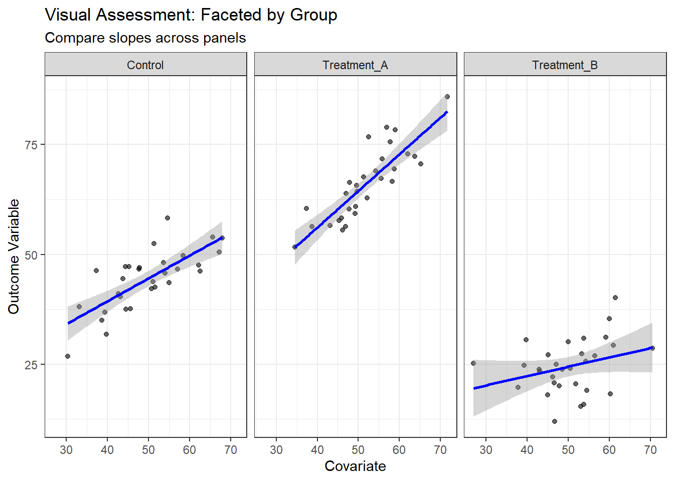

6.5.2.4.3 Method 3: Residuals vs. Covariate Plot

# Fit ANCOVA model (assuming homogeneity)
ancova_model <- lm(outcome ~ Group + covariate, data = data)

# Create residuals plot
data_with_residuals <- data %>%
  mutate(residuals = residuals(ancova_model))

p3 <- ggplot(data_with_residuals, aes(x = covariate, y = residuals, color = Group)) +
  geom_point(alpha = 0.6) +
  geom_smooth(method = "lm", se = FALSE) +
  geom_hline(yintercept = 0, linetype = "dashed") +
  labs(
    title = "Residuals vs. Covariate by Group",
    subtitle = "Non-horizontal lines suggest slope differences",
    x = "Covariate",
    y = "Residuals",
    color = "Group"
  ) +
  scale_color_brewer(type = "qual", palette = "Set1")

print(p3)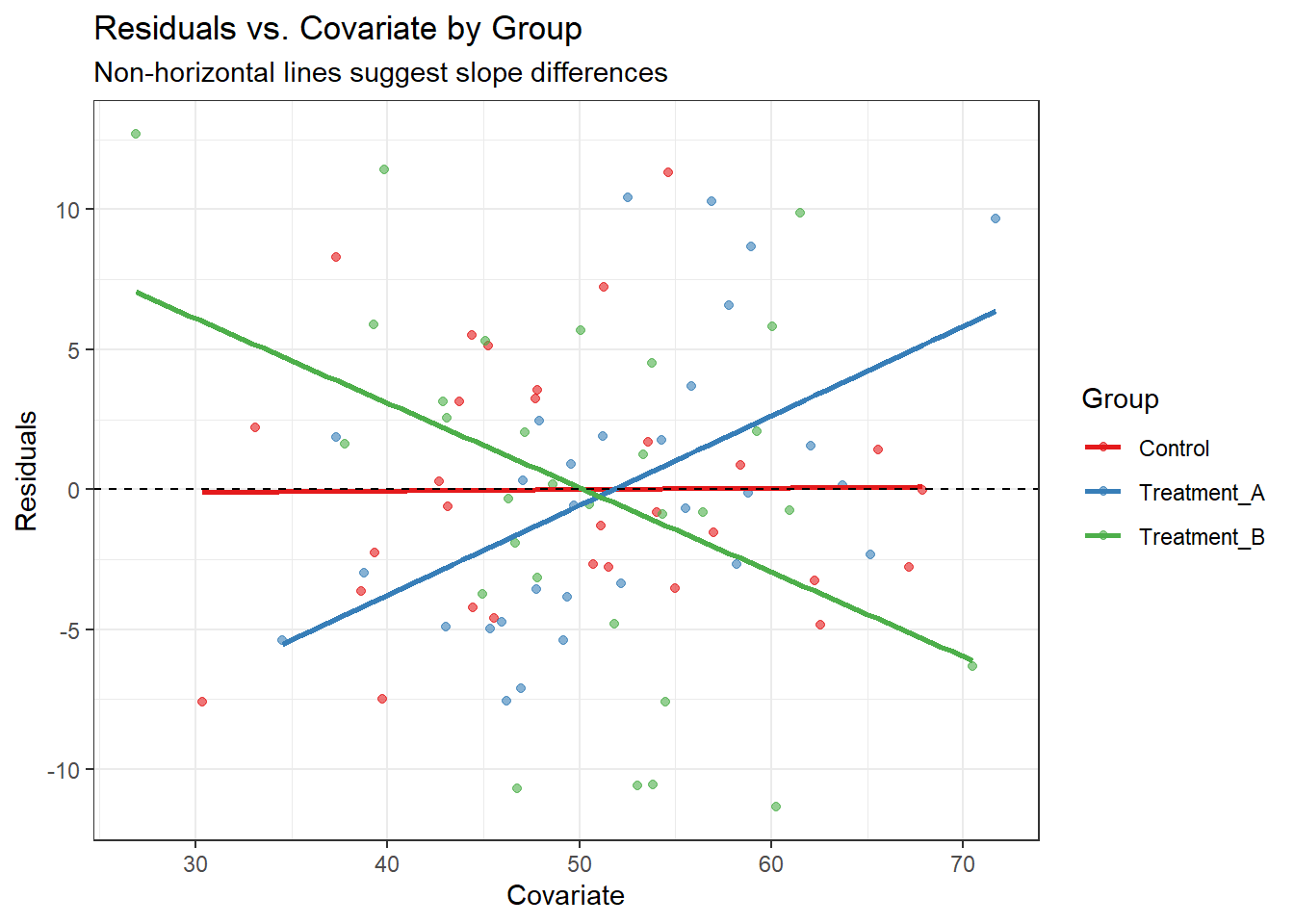

6.5.2.5 Statistical Testing of Homogeneity of Slopes

6.5.2.5.1 Method 1: Testing the Interaction Term

The most direct way to test homogeneity of slopes is to include an interaction term between the factor and covariate:

# Model WITH interaction (allows different slopes)
interaction_model <- lm(outcome ~ Group * covariate, data = data)

# Model WITHOUT interaction (assumes equal slopes - standard ANCOVA)
ancova_model <- lm(outcome ~ Group + covariate, data = data)

# Test the interaction using ANOVA
anova_test <- anova(ancova_model, interaction_model)
print(anova_test)

Analysis of Variance Table

Model 1: outcome ~ Group + covariate
Model 2: outcome ~ Group * covariate
  Res.Df    RSS Df Sum of Sq      F   Pr(>F)    
1     86 2538.1                                 
2     84 2130.2  2    407.83 8.0409 0.000638 ***
---
Signif. codes:  0 '***' 0.001 '**' 0.01 '*' 0.05 '.' 0.1 ' ' 1

# Alternative: Use car package for Type II/III tests
Anova(interaction_model, type = "II")

Anova Table (Type II tests)

Response: outcome
                 Sum Sq Df  F value    Pr(>F)    
Group           24714.1  2 487.2674 < 2.2e-16 ***
covariate        1854.5  1  73.1291 4.741e-13 ***
Group:covariate   407.8  2   8.0409  0.000638 ***
Residuals        2130.2 84                       
---
Signif. codes:  0 '***' 0.001 '**' 0.01 '*' 0.05 '.' 0.1 ' ' 1

6.5.2.5.2 Method 2: Estimate Differences in Slopes

# Get model summaries
slopes1 = avg_slopes(interaction_model,
                     variables = "covariate",
                     by = "Group")
slopes1

       Group Estimate Std. Error    z Pr(>|z|)    S   2.5 % 97.5 %
 Control        0.520     0.0952 5.46   <0.001 24.3 0.33296  0.706
 Treatment_A    0.835     0.1120 7.45   <0.001 43.3 0.61538  1.054
 Treatment_B    0.212     0.1076 1.98   0.0482  4.4 0.00166  0.423

Term: covariate
Type: response
Comparison: dY/dX

slopes1 %>% hypotheses(hypothesis = ~pairwise)

  Hypothesis Estimate Std. Error     z Pr(>|z|)    S   2.5 %  97.5 %
 (b2) - (b1)    0.315      0.147  2.15   0.0319  5.0  0.0273  0.6034
 (b3) - (b1)   -0.307      0.144 -2.14   0.0326  4.9 -0.5887 -0.0255
 (b3) - (b2)   -0.622      0.155 -4.01   <0.001 14.0 -0.9267 -0.3181

6.5.2.6 Diagnostics

6.5.2.6.1 Diagnostic Plots for Both Models

# ANCOVA diagnostic plots

check_model(ancova_model)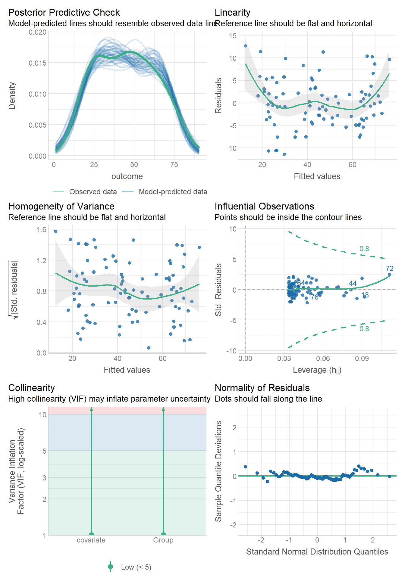

# Interaction model diagnostics
check_model(interaction_model)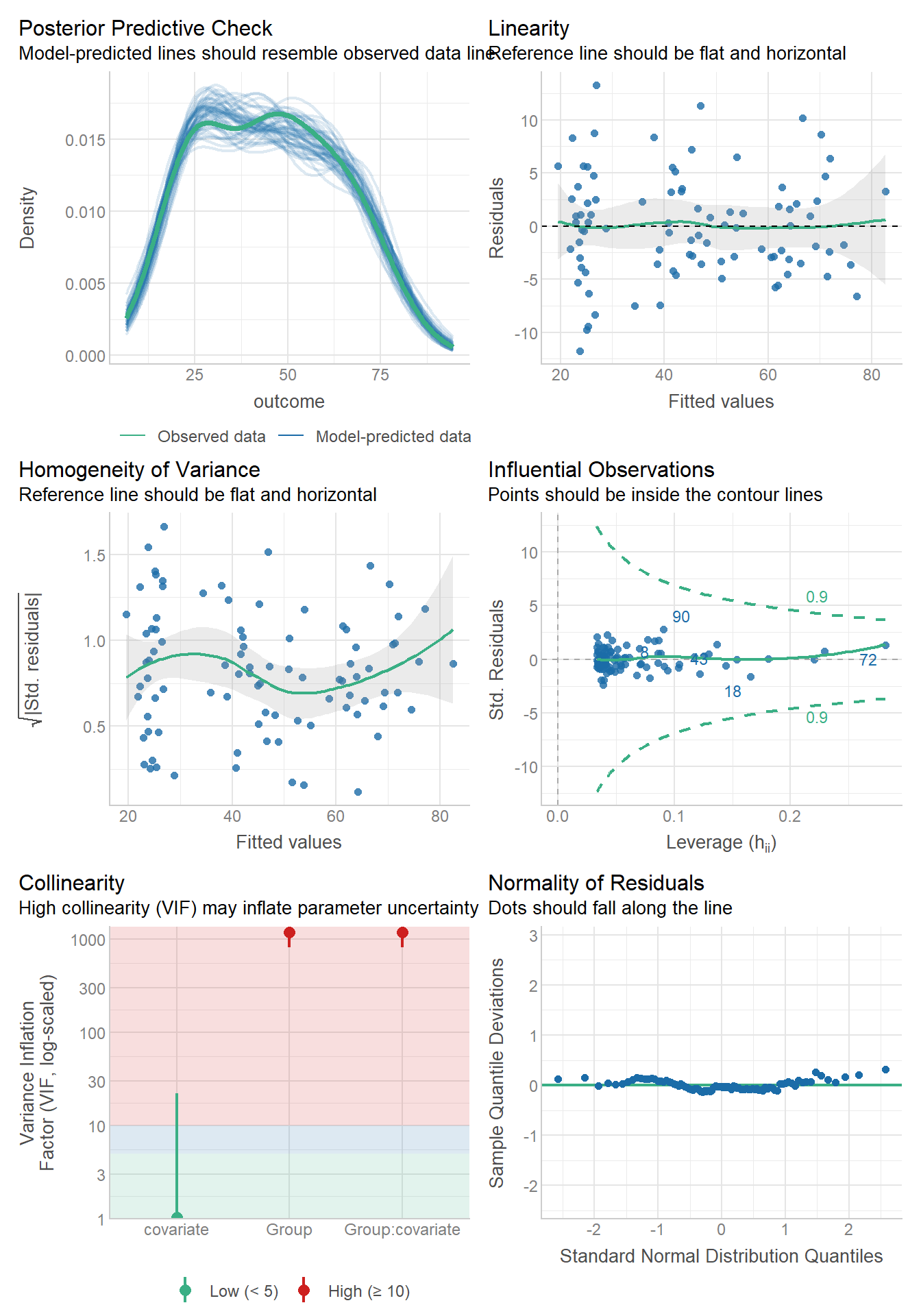

6.5.2.7 Practical Decision Making

6.5.2.7.1 When Homogeneity of Slopes is Violated

We could explore alternative models (it might be that the effects are muliplicative) so we might need to look at log transforming the outcome/covariate.

6.5.2.7.2 Show the Average Marginal Effect

avg_comparisons(interaction_model,
                variable = "Group")

              Contrast Estimate Std. Error     z Pr(>|z|)     S 2.5 % 97.5 %
 Treatment_A - Control     20.1       1.31  15.3   <0.001 174.0  17.5   22.7
 Treatment_B - Control    -20.3       1.30 -15.5   <0.001 178.4 -22.8  -17.7

Term: Group
Type: response

We can also show the distribution underlying the main effect.

comps = comparisons(interaction_model,
                variable = "Group") %>%
  as_tibble()

ggplot(comps,
       aes(x=estimate,group=contrast,fill=contrast))+
    geom_density(adjust=1.5, alpha=.4) +
  facet_wrap(~contrast)+
    theme_bw()

6.5.2.8 Alternative: Johnson-Neyman Technique

When interactions are significant, the Johnson-Neyman technique can identify regions of the covariate where Group differences are significant:

# Using emmeans for Johnson-Neyman analysis
library(modelbased)
slopes <- estimate_slopes(interaction_model, 
                          "Group", 
                          by = "covariate")

plot(slopes)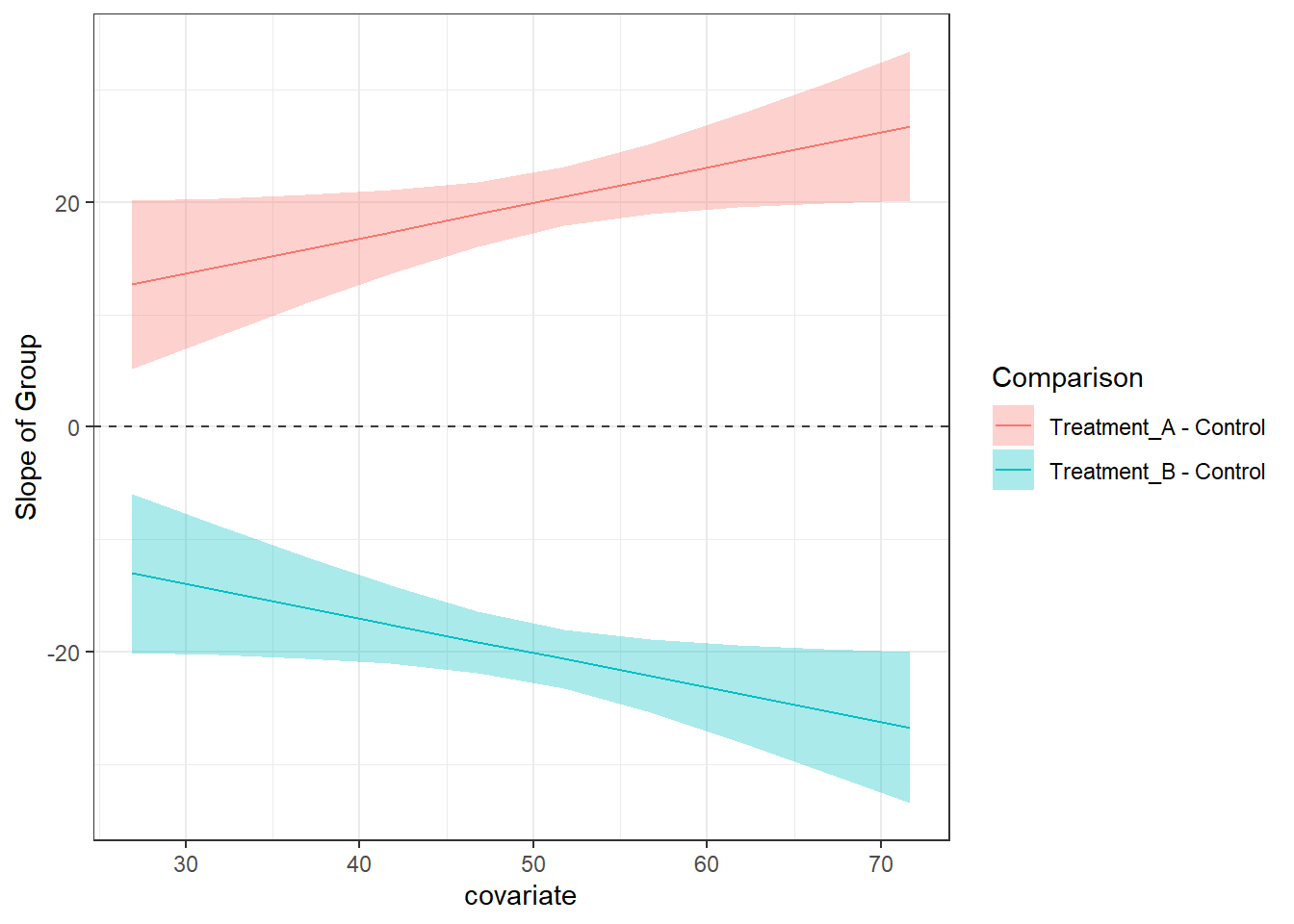

6.5.2.9 Summary and Best Practices

Key Takeaways

1. Always test homogeneity of slopes before interpreting ANCOVA results
2. Visual inspection is crucial - look for parallel lines
3. Statistical testing via interaction terms provides formal evidence
4. When violated, consider using the interaction model or alternative approaches

6.5.3 Application of ANCOVA

In randomized controlled trials with pre-post measurements, we often want to test whether treatments differ in their effects on an outcome variable. Three common approaches are:

1. Post-treatment comparison: Compare groups on post-treatment values only
2. Change score analysis: Compare groups on change from baseline (post - pre)
3. ANCOVA: Use post-treatment as outcome with baseline as covariate

ANCOVA is generally preferred because it:

• Increases statistical power by reducing residual variance
• Provides more precise treatment effect estimates
• Adjusts for any baseline imbalances (even in randomized trials)

6.5.3.1 Data Setup and Simulation

Let’s start by simulating a typical pre-post parallel groups trial dataset:

library(tidyverse)
library(broom)
library(knitr)
library(ggplot2)
library(patchwork)

# Set seed for reproducibility
set.seed(42)

# Simulate pre-post trial data
n_per_group <- 50
n_total <- n_per_group * 2

# Create dataset
trial_data <- tibble(
  id = 1:n_total,
  group = rep(c("Control", "Treatment"), each = n_per_group),
  # Baseline values (normally distributed)
  baseline = rnorm(n_total, mean = 100, sd = 15),
  # Post-treatment values (treatment effect = -10, correlation with baseline = 0.7)
  post = baseline * 0.7 + rnorm(n_total, mean = ifelse(group == "Treatment", 60, 70), sd = 10)
) %>%
  mutate(
    # Calculate change score
    change = post - baseline,
    # Calculate log-transformed values for sympercent analysis
    log_baseline = log(baseline),
    log_post = log(post),
    log_change = log_post - log_baseline
  )

# Display first few rows
head(trial_data) %>% kable(digits = 2)

id	group	baseline	post	change	log_baseline	log_post	log_change
1	Control	120.56	166.40	45.84	4.79	5.11	0.32
2	Control	91.53	144.52	52.99	4.52	4.97	0.46
3	Control	105.45	133.78	28.33	4.66	4.90	0.24
4	Control	109.49	165.13	55.64	4.70	5.11	0.41
5	Control	106.06	137.58	31.51	4.66	4.92	0.26
6	Control	98.41	139.94	41.53	4.59	4.94	0.35

6.5.3.2 Exploratory Data Analysis

Before conducting the analysis, let’s examine our data:

# Summary statistics by group
summary_stats <- trial_data %>%
  group_by(group) %>%
  summarise(
    n = n(),
    baseline_mean = mean(baseline),
    baseline_sd = sd(baseline),
    post_mean = mean(post),
    post_sd = sd(post),
    change_mean = mean(change),
    change_sd = sd(change),
    .groups = 'drop'
  )

summary_stats %>% kable(digits = 2)

group	n	baseline_mean	baseline_sd	post_mean	post_sd	change_mean	change_sd
Control	50	99.46	17.27	138.11	15.99	38.65	10.14
Treatment	50	101.51	13.87	130.82	12.64	29.31	10.06

# Visualizations
p1 <- ggplot(trial_data, aes(x = group, y = baseline, fill = group)) +
  geom_boxplot(alpha = 0.7) +
  labs(title = "Baseline Values by Group", y = "Baseline Score") +
  theme_minimal()

p2 <- ggplot(trial_data, aes(x = group, y = post, fill = group)) +
  geom_boxplot(alpha = 0.7) +
  labs(title = "Post-treatment Values by Group", y = "Post-treatment Score") +
  theme_minimal()

p3 <- ggplot(trial_data, aes(x = baseline, y = post, color = group)) +
  geom_point(alpha = 0.7) +
  geom_smooth(method = "lm", se = TRUE) +
  labs(title = "Baseline vs Post-treatment", 
       x = "Baseline Score", y = "Post-treatment Score") +
  theme_minimal()

p4 <- ggplot(trial_data, aes(x = group, y = change, fill = group)) +
  geom_boxplot(alpha = 0.7) +
  labs(title = "Change Scores by Group", y = "Change Score (Post - Pre)") +
  theme_minimal()

(p1 + p2) / (p3 + p4)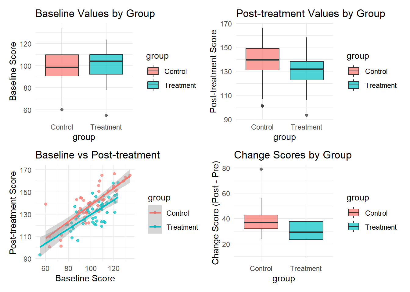

6.5.3.3 Method 1: ANCOVA with Baseline as Covariate

The ANCOVA model treats the post-treatment score as the outcome variable and includes baseline as a covariate:

Model: post ~ group + baseline

# Fit ANCOVA model
ancova_model <- lm(post ~ group + baseline, data = trial_data)

# Model summary
summary(ancova_model)

Call:
lm(formula = post ~ group + baseline, data = trial_data)

Residuals:
     Min       1Q   Median       3Q      Max 
-18.3333  -4.7439   0.3775   4.7490  29.1397 

Coefficients:
            Estimate Std. Error t value Pr(>|t|)    
(Intercept) 62.57031    5.97163  10.478  < 2e-16 ***
group1       4.37815    0.91280   4.796 5.84e-06 ***
baseline     0.71547    0.05873  12.182  < 2e-16 ***
---
Signif. codes:  0 '***' 0.001 '**' 0.01 '*' 0.05 '.' 0.1 ' ' 1

Residual standard error: 9.108 on 97 degrees of freedom
Multiple R-squared:  0.629, Adjusted R-squared:  0.6213 
F-statistic: 82.22 on 2 and 97 DF,  p-value: < 2.2e-16

6.5.3.3.1 Model Diagnostics

# Check model assumptions
check_model(ancova_model)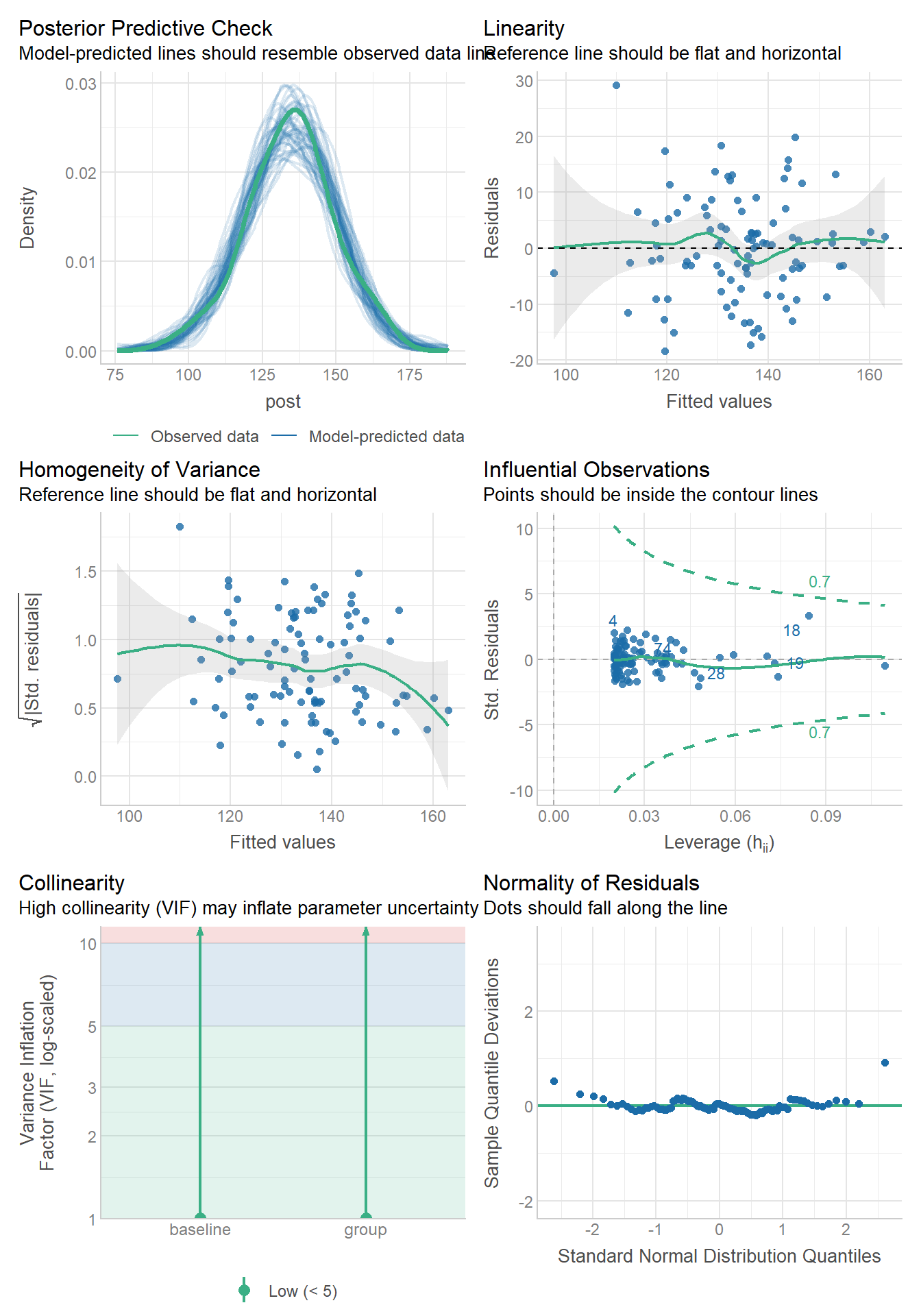

# Test for equal slopes assumption (interaction test)
interaction_model <- lm(post ~ group * baseline, data = trial_data)
anova(ancova_model, interaction_model)

Analysis of Variance Table

Model 1: post ~ group + baseline
Model 2: post ~ group * baseline
  Res.Df    RSS Df Sum of Sq      F Pr(>F)
1     97 8047.1                           
2     96 7985.8  1    61.314 0.7371 0.3927

6.5.3.4 Method 2: Change Score Analysis

An alternative approach is to use the change score (post - pre) as the outcome:

Model: change ~ group

# Fit change score model
change_model <- lm(change ~ group, data = trial_data)

# Model summary
summary(change_model)

Call:
lm(formula = change ~ group, data = trial_data)

Residuals:
    Min      1Q  Median      3Q     Max 
-19.566  -6.567  -0.789   6.121  40.325 

Coefficients:
            Estimate Std. Error t value Pr(>|t|)    
(Intercept)   33.979      1.010  33.647  < 2e-16 ***
group1         4.669      1.010   4.624 1.15e-05 ***
---
Signif. codes:  0 '***' 0.001 '**' 0.01 '*' 0.05 '.' 0.1 ' ' 1

Residual standard error: 10.1 on 98 degrees of freedom
Multiple R-squared:  0.1791,    Adjusted R-squared:  0.1707 
F-statistic: 21.38 on 1 and 98 DF,  p-value: 1.152e-05

emm1 = emmeans(change_model, ~ group)

emm1

 group     emmean   SE df lower.CL upper.CL
 Control     38.6 1.43 98     35.8     41.5
 Treatment   29.3 1.43 98     26.5     32.1

Confidence level used: 0.95 

pairs(emm1)

 contrast            estimate   SE df t.ratio p.value
 Control - Treatment     9.34 2.02 98   4.624  <.0001

6.5.3.4.1 Equivalence of ANCOVA and Change Score

When baseline values are balanced between groups, ANCOVA and change score analysis give similar results. However, ANCOVA is generally more efficient. However, we can use the change score in an ANCOVA!

change_model2 <- lm(change ~ group +
                      baseline, data = trial_data)

pairs(emmeans(ancova_model, ~ group))

 contrast            estimate   SE df t.ratio p.value
 Control - Treatment     8.76 1.83 97   4.796  <.0001

pairs(emmeans(change_model2, ~ group))

 contrast            estimate   SE df t.ratio p.value
 Control - Treatment     8.76 1.83 97   4.796  <.0001

6.5.3.5 Method 3: Log Transformation and Sympercents

When dealing with outcomes that are always positive and may have multiplicative treatment effects, log transformation can be useful. The coefficient from a log-transformed outcome can be interpreted as a “sympercent” (symmetric percent change).

6.5.3.5.1 Understanding Sympercents

When we log-transform both baseline and outcome: - The coefficient represents the log ratio of geometric means - This approximates percent change

# Ensure all values are positive for log transformation


# ANCOVA on log-transformed data
log_ancova <- lm(log_post ~ group + log_baseline, data = trial_data)
summary(log_ancova)

Call:
lm(formula = log_post ~ group + log_baseline, data = trial_data)

Residuals:
      Min        1Q    Median        3Q       Max 
-0.157289 -0.036123  0.002086  0.038943  0.263575 

Coefficients:
             Estimate Std. Error t value Pr(>|t|)    
(Intercept)  2.541260   0.192963  13.170  < 2e-16 ***
group1       0.032711   0.006988   4.681 9.27e-06 ***
log_baseline 0.512055   0.041949  12.206  < 2e-16 ***
---
Signif. codes:  0 '***' 0.001 '**' 0.01 '*' 0.05 '.' 0.1 ' ' 1

Residual standard error: 0.06967 on 97 degrees of freedom
Multiple R-squared:  0.6269,    Adjusted R-squared:  0.6192 
F-statistic: 81.48 on 2 and 97 DF,  p-value: < 2.2e-16

# Extract results
emm1 = emmeans(log_ancova, ~ group)
emm1

 group     emmean      SE df lower.CL upper.CL
 Control    4.928 0.00987 97    4.908    4.947
 Treatment  4.862 0.00987 97    4.843    4.882

Confidence level used: 0.95 

pairs(emm1)

 contrast            estimate    SE df t.ratio p.value
 Control - Treatment   0.0654 0.014 97   4.681  <.0001

6.5.3.5.2 Alternative: Change in Log Values

We can also analyze the change in log values directly:

# Calculate log change score
trial_data <- trial_data %>%
  mutate(log_change = log_post - log_baseline)

# Analyze log change score
log_change_model <- lm(log_change ~ group + log_baseline, data = trial_data)
summary(log_change_model)

Call:
lm(formula = log_change ~ group + log_baseline, data = trial_data)

Residuals:
      Min        1Q    Median        3Q       Max 
-0.157289 -0.036123  0.002086  0.038943  0.263575 

Coefficients:
              Estimate Std. Error t value Pr(>|t|)    
(Intercept)   2.541260   0.192963  13.170  < 2e-16 ***
group1        0.032711   0.006988   4.681 9.27e-06 ***
log_baseline -0.487945   0.041949 -11.632  < 2e-16 ***
---
Signif. codes:  0 '***' 0.001 '**' 0.01 '*' 0.05 '.' 0.1 ' ' 1

Residual standard error: 0.06967 on 97 degrees of freedom
Multiple R-squared:  0.6322,    Adjusted R-squared:  0.6246 
F-statistic: 83.37 on 2 and 97 DF,  p-value: < 2.2e-16

emm1 = emmeans(log_change_model, ~ group)
emm1

 group     emmean      SE df lower.CL upper.CL
 Control    0.331 0.00987 97    0.311    0.351
 Treatment  0.266 0.00987 97    0.246    0.285

Confidence level used: 0.95 

pairs(emm1)

 contrast            estimate    SE df t.ratio p.value
 Control - Treatment   0.0654 0.014 97   4.681  <.0001

6.5.3.6 Key Takeaways

1. ANCOVA with baseline covariate is generally preferred for pre-post trial analysis because:

   • It provides more precise estimates (smaller standard errors)
   • It adjusts for baseline imbalances
   • It increases statistical power

2. Change score analysis gives similar point estimates but is less efficient

• You can include change scores as the outcome
• It will be statistically equivalent to the ANCOVA on post scores
• Interpretation might be different, a good compromise
• Caution is still warranted as things get wonky with change scores, preferrably to use post scores when possible.

3. Log transformation is useful when:

   • The outcome is always positive
   • Treatment effects are multiplicative rather than additive
   • You want to interpret results as percent changes

4. Sympercents (coefficients from log-transformed outcomes) can be a way to interpret results as a percent difference

5. Model assumptions should always be checked, particularly:

   • Equal slopes assumption for ANCOVA (test group × baseline interaction)
   • Normality and homoscedasticity of residuals
   • For log transformation: positive of all values (zero not possible)

6.5.3.7 References and Further Reading

• Senn, S. (2006). Change from baseline and analysis of covariance revisited. Statistics in Medicine, 25(24), 4334-4344.
• Vickers, A. J., & Altman, D. G. (2001). Analysing controlled trials with baseline and follow up measurements. BMJ, 323(7321), 1123-1124.