# Here are the libraries I used
library(tidyverse) # standard
library(knitr) # need for a couple things to make knitted document to look nice
library(readr) # need to read in data
library(ggpubr) # allows for stat_cor in ggplots
library(ggfortify) # Needed for autoplot to work on lm()
library(gridExtra) # allows me to organize the graphs in a grid
library(car) # need for some regression stuff like vif
library(GGally)
library(Hmisc) # Needed for some visuals
library(rms) # needed for some data reduction tech.
library(pcaPP)
library(see)
library(performance)4 Module 4: Multiple Regression
Here are some code chunks that setup this chapter
# This changes the default theme of ggplot
old.theme <- theme_get()
theme_set(theme_bw())
4.1 SENIC Data
We will now begin the examining data from the Study on the Efficcacy of Nosocomial Infection Control (SENIC project). The general objective, and therefore project name, was to examine how effective infection surveillance and control programs were at reducing hopsital acquired (nosocomial) diseases. Data was obtained through the test Applied Linear Statistical Models 5th edition (Neter et al).
senic <- read_csv(here::here("datasets",
'SENIC.csv'))stayLength: Average length of stay of all patients in hospital (in days)age: Average age of patients (in years)infectionRisk: Average estimated probability of acquiring infection in hospital (in percent)cultureRatio: Ratio of number of cultures performed to number of patients without signs or symptoms of hospital-acquired infection, times 100xrayRatio: Ratio of number of X-rays performed to number of patients , without signs or symptoms of pneumonia, times 100beds: Average number of beds in hospital during study periodschoolMed school affiliation (Yes or No)region: Geographic region (NE, NC, S, W)patients: Average number of patients in hospital per day during study periodnurses: Average number of full-time equivalent registered and licensed practical nurses during study period (number full-time plus one half the number part time)facilities: Percent of 35 potential facilities and services that are provided by the hospital
4.2 Infection Risk
There are a lot of potential variables that may relate to infectionRisk, but let’s just concentrate on stayLength and cultureRatio.
#isc ending indicates the variables used:
#(i)nfectionRisk, (s)tayLength, (c)ultureRatio

senicisc <- select(senic, infectionRisk,
                   stayLength, cultureRatio)
4.2.1 Relation of infectionRisk with stayLength and cultureRatio
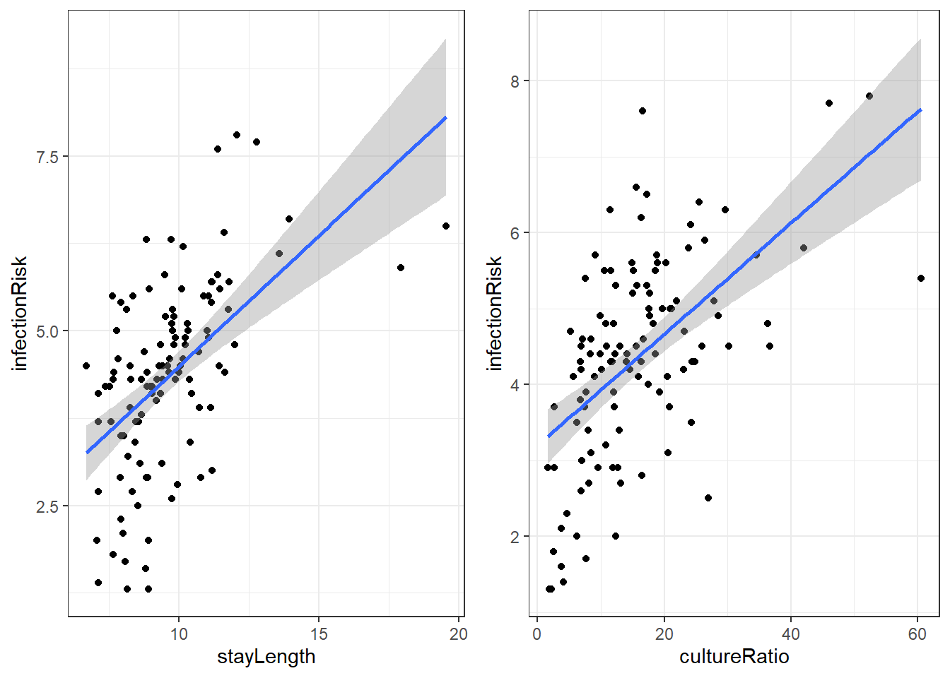
4.2.2 Model with stayLength
Here is the linear regression output for infectionRisk with stayLength.
infStayLm <- lm(infectionRisk ~ stayLength, senicisc)
summary(infStayLm)
Call:
lm(formula = infectionRisk ~ stayLength, data = senicisc)

Residuals:
    Min      1Q  Median      3Q     Max
-2.7823 -0.7039  0.1281  0.6767  2.5859

Coefficients:
            Estimate Std. Error t value Pr(>|t|)
(Intercept)  0.74430    0.55386   1.344    0.182
stayLength   0.37422    0.05632   6.645 1.18e-09 ***
---
Signif. codes:  0 '***' 0.001 '**' 0.01 '*' 0.05 '.' 0.1 ' ' 1

Residual standard error: 1.139 on 111 degrees of freedom
Multiple R-squared:  0.2846,    Adjusted R-squared:  0.2781
F-statistic: 44.15 on 1 and 111 DF,  p-value: 1.177e-09
Our regression equation for predicting infectionRisk is:
\[\widehat{risk} = 0.744 + 0.374\cdot stayLength\]
4.2.3 Model with cultureRatio
Here is the linear regression output for infectionRisk with cultureRatio.
infCuLm <- lm(infectionRisk ~ cultureRatio, senicisc)
summary(infCuLm)
Call:
lm(formula = infectionRisk ~ cultureRatio, data = senicisc)

Residuals:
    Min      1Q  Median      3Q     Max
-2.6759 -0.7133  0.1593  0.7966  3.1860

Coefficients:
             Estimate Std. Error t value Pr(>|t|)
(Intercept)   3.19790    0.19377  16.504  < 2e-16 ***
cultureRatio  0.07326    0.01031   7.106 1.22e-10 ***
---
Signif. codes:  0 '***' 0.001 '**' 0.01 '*' 0.05 '.' 0.1 ' ' 1

Residual standard error: 1.117 on 111 degrees of freedom
Multiple R-squared:  0.3127,    Adjusted R-squared:  0.3065
F-statistic: 50.49 on 1 and 111 DF,  p-value: 1.218e-10
The regression equation is then:
\[\widehat{risk} = 3.198 + 0.073\cdot cultureRatio\]
4.3 Linear Regression with Two Variables
We can “easily” create a model that accounts for a linear relationship between two variables. If we have one response variable \(y\) and two predictor variables \(x_1\) and \(x_2\), then the model is:
\[y = \beta_0 + \beta_1 x_1 + \beta_2 x_2 + \epsilon\]
Where we assume that we have error terms \(\epsilon \sim N(0,\sigma_\epsilon)\) which are independent. An additional assumption is that the two predictor variables, \(x_1\) and \(x_2\) are independent of each other.
We still have two parts to the model.
- The linear relation/conditional mean \(\mu_{y|x} = \beta_0 + \beta_1 x_1 + \beta_2 x_2\)
- The error \(\epsilon\)
4.4 Model for infectionRisk using two variables
The way to get the estimated regression equation is the same. We just add another variable into the lm() formula.
riskLm <- lm(infectionRisk ~ stayLength + cultureRatio,
             data=senicisc)

summary(riskLm)
Call:
lm(formula = infectionRisk ~ stayLength + cultureRatio, data = senicisc)
Residuals:
Min 1Q Median 3Q Max
-2.1822 -0.7275 0.1040 0.6847 2.7143
Coefficients:
Estimate Std. Error t value Pr(>|t|)
(Intercept) 0.805491 0.487756 1.651 0.102
stayLength 0.275472 0.052465 5.251 7.46e-07 ***
cultureRatio 0.056451 0.009798 5.761 7.70e-08 ***
---
Signif. codes: 0 '***' 0.001 '**' 0.01 '*' 0.05 '.' 0.1 ' ' 1
Residual standard error: 1.003 on 110 degrees of freedom
Multiple R-squared: 0.4504, Adjusted R-squared: 0.4404
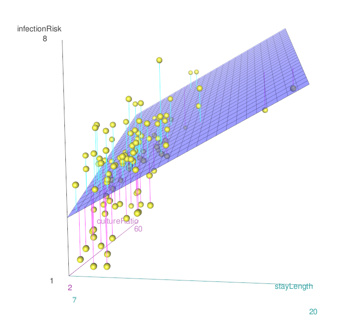
F-statistic: 45.07 on 2 and 110 DF, p-value: 5.04e-15So our model for estimated risk is
\[\widehat{risk} = 0.805 + 0.275 \cdot stayLength + 0.056\cdot cultureRatio\]
4.4.1 Graphing the relationship
4.4.2 Interpreting the Coefficients
The interpretation, so now we have to figure out to interpret three different estimated coefficients: \(\widehat \beta_{0}, \widehat \beta_{1}, \widehat \beta_{2}\).
\(\widehat \beta_{0}\) is the estimated y-intercept. The idea behind the intercept coefficient is similar, except for now it is \(\hat \mu_{y|x}hat\), the estimated mean value of the \(y\) variable, when both \(x_1\) and \(x_2\) are 0.
\(\widehat \beta_{1}\) is the amount that \(\hat \mu_{y|x}\) increases when \(x_1\) increases by 1 unit AND \(x_2\) is constant.
\(\widehat \beta_{2}\) is the amount that \(\hat \mu_{y|x}\) increases when \(x_2\) increases by 1 unit AND \(x_1\) is constant.
So for our estimated regression model:
\[\widehat{risk} = 0.805 + 0.275 \cdot stayLength + 0.056\cdot cultureRatio\]
We estimate that the mean infection risk of hospitals is 0.805% among hospitals with an average length of stay if 0 days and average culture ratio of 0. (Does this make sense?)
We estimate that the mean infection risk of hospitals increases by 0.275% among hospitals with average length of stay 1 day longer, and average culture ratio saying constant.
We estimate that the mean infection risk of hospitals increases by 0.056% among hospitals where the average culture ratio rate is 1 unit higher, and average length of stay remains constant.
4.5 Inference on the regression coefficients
Just like before, there are several columns for each coefficient. The columns are for the following hypothesis test.
\[H_0: \beta_k = 0\] \[H_1: \beta_k \ne 0\]
The test statistic is:
\[t = \frac{\hat \beta_k}{SE_{\hat \beta_k}}\]
We simple divide our coefficient estimate by its standard error.
The test statistic is assumed to be from a \(t\) distribution with degrees of freedom \(df = n - (p+1)\). Where \(p\) is the total number of predictor variables. And the p-value is the probability of obtaining
When looking at our model summary we interpret the p-values similarly.
summary(riskLm)
Call:
lm(formula = infectionRisk ~ stayLength + cultureRatio, data = senicisc)

Residuals:
    Min      1Q  Median      3Q     Max
-2.1822 -0.7275  0.1040  0.6847  2.7143

Coefficients:
             Estimate Std. Error t value Pr(>|t|)
(Intercept)  0.805491   0.487756   1.651    0.102
stayLength   0.275472   0.052465   5.251 7.46e-07 ***
cultureRatio 0.056451   0.009798   5.761 7.70e-08 ***
---
Signif. codes:  0 '***' 0.001 '**' 0.01 '*' 0.05 '.' 0.1 ' ' 1

Residual standard error: 1.003 on 110 degrees of freedom
Multiple R-squared:  0.4504,    Adjusted R-squared:  0.4404
F-statistic: 45.07 on 2 and 110 DF, p-value: 5.04e-15- There is weak evidence that the true linear model has a non-zero intercept.
- There is extremely strong evidence that there is a linear component in the relationship between
stayLengthandinfectionRisk(\(p<0.0001\)) whencultureRatiois included in the model. - There is extremely strong evidence that there is a linear component in the relationship between
cultureRatioandinfectionRisk(\(p<0.0001\)) whenstayLengthis included in the model.
The test for the intercept is not important (usually). The tests for the slopes are more important though not terribly so by themselves.
4.6 Understanding the Difference in Nominal Significance Error (DINS)
4.6.1 What is DINS?
The Difference in Nominal Significance Error (DINS) occurs when we incorrectly conclude that two regression coefficients differ significantly from each other based solely on their individual statistical significance tests. In simpler terms, we make this error when we observe:
- Coefficient A is statistically significant (p < 0.05)
- Coefficient B is not statistically significant (p > 0.05)
- We then incorrectly conclude that A and B must be significantly different from each other
4.6.2 Why is this an error?
This reasoning is flawed because the difference between “significant” and “not significant” is not itself necessarily significant. Two coefficients can have different p-values (one below 0.05 and one above 0.05), yet the difference between the coefficients themselves might not be statistically significant.
4.6.3 How to properly compare coefficients
To correctly determine if two coefficients differ significantly:
- Calculate the difference between the coefficients
- Calculate the standard error of this difference
- Perform a formal hypothesis test on this difference
- Or construct a confidence interval for the difference
4.6.4 Example in multiple regression
Consider a regression model with two predictors X_1_ and X_2_:
\[ Y = \beta_0 + \beta_1X_1 + \beta_2X_2 + \epsilon \]
If Beta1 = 0.5 with p = 0.03 (significant) and Beta2 = 0.3 with p = 0.08 (not significant), we cannot automatically conclude that Beta1 is significantly different from Beta2. We need to explicitly test whether Beta1- Beta2 differs significantly from zero.
4.6.5 Example of a test
Both significant… and significantly different… but does that matter?!?
We could normalize to the SD of the predictor… but does is that matter!?!
Let’s consider a model from earlier…
summary(riskLm)
Call:
lm(formula = infectionRisk ~ stayLength + cultureRatio, data = senicisc)

Residuals:
    Min      1Q  Median      3Q     Max
-2.1822 -0.7275  0.1040  0.6847  2.7143

Coefficients:
             Estimate Std. Error t value Pr(>|t|)
(Intercept)  0.805491   0.487756   1.651    0.102
stayLength   0.275472   0.052465   5.251 7.46e-07 ***
cultureRatio 0.056451   0.009798   5.761 7.70e-08 ***
---
Signif. codes:  0 '***' 0.001 '**' 0.01 '*' 0.05 '.' 0.1 ' ' 1

Residual standard error: 1.003 on 110 degrees of freedom
Multiple R-squared:  0.4504,    Adjusted R-squared:  0.4404
F-statistic: 45.07 on 2 and 110 DF, p-value: 5.04e-15library(marginaleffects)
# Coefficients
avg_comparisons(riskLm)
         Term Estimate Std. Error    z Pr(>|z|)    S  2.5 % 97.5 %
 cultureRatio   0.0565     0.0098 5.76   <0.001 26.8 0.0372 0.0757
 stayLength     0.2755     0.0525 5.25   <0.001 22.7 0.1726 0.3783

Type: response
Comparison: +1
# Compare Coefficients
avg_comparisons(riskLm,
hypothesis = "cultureRatio = stayLength")
              Hypothesis Estimate Std. Error     z Pr(>|z|)    S 2.5 % 97.5 %
 cultureRatio=stayLength   -0.219     0.0564 -3.88   <0.001 13.2 -0.33 -0.108

Type: response
# Compare Standardized Coefficients using Marginal Effects
avg_comparisons(riskLm,
variables = list(cultureRatio = "sd",
stayLength = "sd"))
         Term Estimate Std. Error    z Pr(>|z|)    S 2.5 % 97.5 %
 cultureRatio    0.578        0.1 5.76   <0.001 26.8 0.381  0.774
 stayLength      0.527        0.1 5.25   <0.001 22.7 0.330  0.723

Type: response
Comparison: (x + sd/2) - (x - sd/2)avg_comparisons(
riskLm,
variables = list(cultureRatio = "sd", stayLength = "sd"),
hypothesis = "cultureRatio = stayLength"
)
              Hypothesis Estimate Std. Error     z Pr(>|z|)   S  2.5 % 97.5 %
 cultureRatio=stayLength   0.0512      0.163 0.313    0.754 0.4 -0.269  0.371

Type: response
4.6.6 Implications for interpretation
When interpreting multiple regression coefficients:
- Avoid comparing significance levels directly
- Use proper statistical tests for coefficient differences
- Consider scale of the predictor and what your research question is!
Recognizing and avoiding the DINS error helps ensure your statistical conclusions are valid and well-supported by your data.
4.7 Categorical and Ordinal Variables in Regression Models
4.7.1 Introduction
In regression analysis, predictor variables can be:
- Continuous: Numerical variables that can take any value within a range (e.g., age, income, temperature)
- Categorical: Variables with distinct categories or groups (e.g., gender, color, treatment type)
- Ordinal: Categorical variables with a natural ordering (e.g., education level, satisfaction rating)
4.7.2 Categorical Variables (Nominal)
4.7.2.1 Key Characteristics
- No inherent ordering between categories
- Examples: gender (male/female), color (red/blue/green), treatment (A/B/C)
- Cannot be used directly in regression as numerical values
4.7.2.2 Dummy Variable Encoding
To include categorical variables in regression, we create dummy variables (also called indicator variables):
# Example: Color variable with 3 categories (red, blue, green)
data <- data.frame(
  y = c(10, 15, 12, 18, 14, 16),
  color = c("red", "blue", "green",
            "red", "blue", "green")
)

# Create dummy variables manually
data$color_blue <- ifelse(data$color == "blue", 1, 0)
data$color_green <- ifelse(data$color == "green", 1, 0)
# Note: red is the reference category (omitted)

# Or use R's factor system (automatic dummy creation)
data$color <- factor(data$color)
model <- lm(y ~ color, data = data)
summary(model)
Call:
lm(formula = y ~ color, data = data)

Residuals:
   1    2    3    4    5    6
-4.0  0.5 -2.0  4.0 -0.5  2.0

Coefficients:
            Estimate Std. Error t value Pr(>|t|)
(Intercept)   14.500      2.598   5.581   0.0114 *
colorgreen    -0.500      3.674  -0.136   0.9004
colorred      -0.500      3.674  -0.136   0.9004
---
Signif. codes:  0 '***' 0.001 '**' 0.01 '*' 0.05 '.' 0.1 ' ' 1

Residual standard error: 3.674 on 3 degrees of freedom
Multiple R-squared:  0.008163,  Adjusted R-squared:  -0.6531
F-statistic: 0.01235 on 2 and 3 DF,  p-value: 0.9878
4.7.2.3 Reference Category
- One category is always omitted as the reference category
- Coefficients represent the difference from the reference category
- R automatically chooses the first alphabetical category as reference
# Change reference category
data$color <- relevel(factor(data$color), ref = "blue")
model2 <- lm(y ~ color, data = data)
4.7.3 Ordinal Variables
4.7.3.1 Key Characteristics
- Categories have a natural ordering
- Examples: education (high school < bachelor’s < master’s < PhD), satisfaction (low < medium < high)
- Can be treated as categorical OR utilize the ordering information
4.7.3.2 Approach 1: Treat as Categorical
# Create example dataset with ordinal variable
set.seed(123)
n <- 100

# Create ordinal education variable
education_levels <- c("High School", "Some College", "Bachelor", "Graduate")
data <- data.frame(
  salary = rnorm(n, 50000, 15000),
  education = sample(education_levels, n, replace = TRUE),
  experience = runif(n, 0, 20)
)

# Method 1: Treat as regular categorical (dummy variables)
data$education_cat <- factor(data$education)
model_cat <- lm(salary ~ education_cat + experience, data = data)
summary(model_cat)
Call:
lm(formula = salary ~ education_cat + experience, data = data)

Residuals:
   Min     1Q Median     3Q    Max
-32390  -9723   -886   9345  32913

Coefficients:
                          Estimate Std. Error t value Pr(>|t|)
(Intercept)                46414.8     3764.9  12.328   <2e-16 ***
education_catGraduate       6697.0     4127.6   1.622    0.108
education_catHigh School    -824.6     3988.1  -0.207    0.837
education_catSome College   1775.5     4164.3   0.426    0.671
experience                   315.4      238.6   1.322    0.189
---
Signif. codes:  0 '***' 0.001 '**' 0.01 '*' 0.05 '.' 0.1 ' ' 1

Residual standard error: 13560 on 95 degrees of freedom
Multiple R-squared:  0.05917,   Adjusted R-squared:  0.01955
F-statistic: 1.494 on 4 and 95 DF,  p-value: 0.2103
4.7.3.3 Approach 2: Ordered Factors
# Method 2: Ordered factor with polynomial contrasts
data$education_ord <- factor(data$education,
                            levels = c("High School", "Some College",
                                     "Bachelor", "Graduate"),
                            ordered = TRUE)

model_ord <- lm(salary ~ education_ord + experience, data = data)
summary(model_ord)
Call:
lm(formula = salary ~ education_ord + experience, data = data)

Residuals:
   Min     1Q Median     3Q    Max
-32390  -9723   -886   9345  32913

Coefficients:
                Estimate Std. Error t value Pr(>|t|)
(Intercept)      48326.8     2680.9  18.026   <2e-16 ***
education_ord.L   4648.6     2627.4   1.769    0.080 .
education_ord.Q   2048.5     2794.0   0.733    0.465
education_ord.C   2872.9     2914.1   0.986    0.327
experience         315.4      238.6   1.322    0.189
---
Signif. codes:  0 '***' 0.001 '**' 0.01 '*' 0.05 '.' 0.1 ' ' 1

Residual standard error: 13560 on 95 degrees of freedom
Multiple R-squared:  0.05917,   Adjusted R-squared:  0.01955
F-statistic: 1.494 on 4 and 95 DF,  p-value: 0.2103
4.7.3.4 Approach 3: Set a different contrast coding
Proceed with caution
# Method 3: Manual contrast coding
contrasts(data$education_cat) = contr.helmert(4)
model_num <- lm(salary ~ education_cat + experience, data = data)
summary(model_num)
Call:
lm(formula = salary ~ education_cat + experience, data = data)

Residuals:
   Min     1Q Median     3Q    Max
-32390  -9723   -886   9345  32913

Coefficients:
               Estimate Std. Error t value Pr(>|t|)
(Intercept)    48326.83    2680.91  18.026   <2e-16 ***
education_cat1  3348.52    2063.82   1.622    0.108
education_cat2 -1391.04    1075.88  -1.293    0.199
education_cat3   -45.49     802.99  -0.057    0.955
experience       315.40     238.60   1.322    0.189
---
Signif. codes:  0 '***' 0.001 '**' 0.01 '*' 0.05 '.' 0.1 ' ' 1

Residual standard error: 13560 on 95 degrees of freedom
Multiple R-squared:  0.05917,   Adjusted R-squared:  0.01955
F-statistic: 1.494 on 4 and 95 DF,  p-value: 0.2103
4.7.4 Key Considerations
4.7.4.1 Model Interpretation
- Categorical coefficients: Difference in outcome between that category and reference category
- Ordinal coefficients:
- Linear term: overall linear trend across ordered categories
- Quadratic term: curvature in the relationship
- Higher-order terms: more complex patterns
4.7.4.2 Choosing the Approach
- Use categorical approach when ordering is not meaningful or you want maximum flexibility
- Use ordinal approach when ordering is meaningful and you want to capture trends
- Be cautious with custom contrasts unless you’re confident about your interpretation
4.7.5 Degrees of Freedom
- Categorical variable with k categories uses k-1 degrees of freedom
- Ordinal polynomial contrasts also use k-1 degrees of freedom but partition them into trend components
4.7.6 Summary
- Categorical variables require dummy variable encoding for regression
- Reference category interpretation is crucial
- Ordinal variables offer multiple encoding options depending on research goals
- Always examine your contrasts and ensure they align with your research questions
- R’s factor system handles much of the encoding automatically, but understanding the underlying mechanics is essential for proper interpretation
4.8 Interaction Terms in Regression Models
4.8.1 What are Interaction Terms?
In regression analysis, an interaction term allows the effect of one predictor variable to depend on the value of another predictor variable. Without interactions, we assume that predictors have independent, additive effects on the outcome.
4.8.1.1 Mathematical Foundation
Additive Model (No Interaction): \(Y = \beta_0 + \beta_1 X_1 + \beta_2 X_2 + \varepsilon\)
Model with Interaction: \(Y = \beta_0 + \beta_1 X_1 + \beta_2 X_2 + \beta_3(X_1 \times X_2) + \varepsilon\)
The interaction coefficient \(\beta_3\) tells us how much the effect of \(X_1\) on \(Y\) changes for each one-unit increase in \(X_2\).
4.8.2 The Parallel Slopes Concept
4.8.2.1 Without Interaction (Parallel Slopes)
When there’s no interaction between a continuous and categorical variable, the regression lines for different groups have the same slope but different intercepts - they are parallel.
# Example: No interaction between income and education level
model_additive <- lm(salary ~ income + education_level, data = df)
4.8.2.2 With Interaction (Non-Parallel Slopes)
When an interaction exists, the slopes differ between groups - the lines are not parallel.
# Example: Interaction between income and education level
model_interaction <- lm(salary ~ income * education_level, data = df)
# Note: income * education_level expands to:
# income + education_level + income:education_level
4.8.3 Types of Interactions
4.8.3.1 1. Continuous × Categorical Interaction
# Load example data
library(ggplot2)
data(mtcars)

# Create interaction model: mpg predicted by weight and transmission type
model <- lm(mpg ~ wt * am, data = mtcars)
summary(model)
Call:
lm(formula = mpg ~ wt * am, data = mtcars)

Residuals:
    Min      1Q  Median      3Q     Max
-3.6004 -1.5446 -0.5325  0.9012  6.0909

Coefficients:
            Estimate Std. Error t value Pr(>|t|)
(Intercept)  31.4161     3.0201  10.402 4.00e-11 ***
wt           -3.7859     0.7856  -4.819 4.55e-05 ***
am           14.8784     4.2640   3.489  0.00162 **
wt:am        -5.2984     1.4447  -3.667  0.00102 **
---
Signif. codes:  0 '***' 0.001 '**' 0.01 '*' 0.05 '.' 0.1 ' ' 1

Residual standard error: 2.591 on 28 degrees of freedom
Multiple R-squared:  0.833, Adjusted R-squared:  0.8151
F-statistic: 46.57 on 3 and 28 DF,  p-value: 5.209e-11
# Visualize the interaction
ggplot(mtcars, aes(x = wt, y = mpg, color = factor(am))) +
geom_point() +
geom_smooth(method = "lm", se = FALSE) +
labs(x = "Weight (1000 lbs)",
y = "Miles per Gallon",
color = "Transmission\n(0=Auto, 1=Manual)") +
theme_minimal()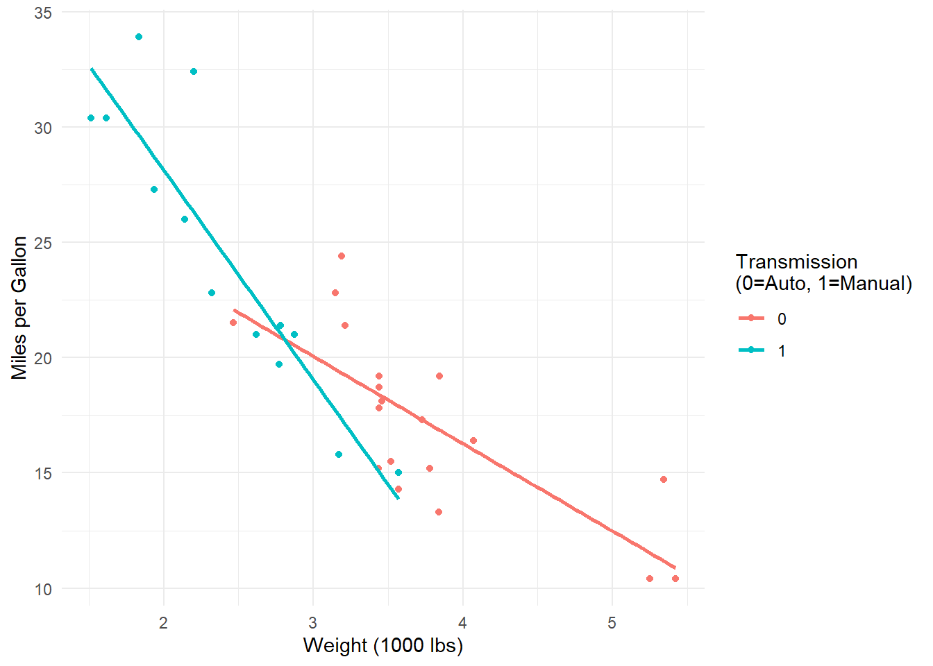
Interpretation: The effect of weight on fuel efficiency differs between automatic and manual transmissions.
4.8.3.2 2. Continuous × Continuous Interaction
# Example with two continuous variables
model_cont <- lm(mpg ~ wt * hp, data = mtcars)
summary(model_cont)
Call:
lm(formula = mpg ~ wt * hp, data = mtcars)

Residuals:
    Min      1Q  Median      3Q     Max
-3.0632 -1.6491 -0.7362  1.4211  4.5513

Coefficients:
            Estimate Std. Error t value Pr(>|t|)
(Intercept) 49.80842    3.60516  13.816 5.01e-14 ***
wt          -8.21662    1.26971  -6.471 5.20e-07 ***
hp          -0.12010    0.02470  -4.863 4.04e-05 ***
wt:hp        0.02785    0.00742   3.753 0.000811 ***
---
Signif. codes:  0 '***' 0.001 '**' 0.01 '*' 0.05 '.' 0.1 ' ' 1

Residual standard error: 2.153 on 28 degrees of freedom
Multiple R-squared:  0.8848,    Adjusted R-squared:  0.8724
F-statistic: 71.66 on 3 and 28 DF,  p-value: 2.981e-13
# The interaction term wt:hp tells us how the effect of weight
# changes as horsepower increases (or vice versa)4.8.3.3 3. Categorical × Categorical Interaction
# Example with factors
model_cat <- lm(mpg ~ factor(cyl) * factor(am), data = mtcars)
summary(model_cat)
Call:
lm(formula = mpg ~ factor(cyl) * factor(am), data = mtcars)

Residuals:
    Min      1Q  Median      3Q     Max
-6.6750 -1.1000  0.1125  1.6875  5.8250

Coefficients:
                         Estimate Std. Error t value Pr(>|t|)
(Intercept)                22.900      1.751  13.081 6.06e-13 ***
factor(cyl)6               -3.775      2.316  -1.630 0.115155
factor(cyl)8               -7.850      1.957  -4.011 0.000455 ***
factor(am)1                 5.175      2.053   2.521 0.018176 *
factor(cyl)6:factor(am)1   -3.733      3.095  -1.206 0.238553
factor(cyl)8:factor(am)1   -4.825      3.095  -1.559 0.131069
---
Signif. codes:  0 '***' 0.001 '**' 0.01 '*' 0.05 '.' 0.1 ' ' 1

Residual standard error: 3.032 on 26 degrees of freedom
Multiple R-squared:  0.7877,    Adjusted R-squared:  0.7469
F-statistic: 19.29 on 5 and 26 DF,  p-value: 5.179e-08
4.8.4 Interpreting Interaction Coefficients
Consider the model: \(Y = \beta_0 + \beta_1 X_1 + \beta_2 X_2 + \beta_3(X_1 \times X_2)\)
4.8.4.1 For Continuous × Categorical:
- \(\beta_1\): Effect of \(X_1\) when \(X_2 = 0\) (reference category)
- \(\beta_2\): Difference in intercept between categories when \(X_1 = 0\)
- \(\beta_3\): How much the slope of \(X_1\) differs between categories
4.8.4.2 Example Interpretation:
# If our model is: salary ~ experience * gender
# Where gender: 0 = male, 1 = female

# Coefficients might be:
# (Intercept): 40000  - Starting salary for males with 0 experience
# experience:   2000  - Salary increase per year experience for males
# gender:       5000  - Salary difference for females at 0 experience
# experience:gender: -500 - How much less the experience effect is for females

# This means:
# Males: salary = 40000 + 2000(experience)
# Females: salary = 45000 + 1500(experience)
4.9 Practical Example in R
# Complete example with interpretation
library(ggplot2)

# Simulate data
set.seed(123)
n <- 100
experience <- runif(n, 0, 20)
gender <- rbinom(n, 1, 0.5)  # 0 = male, 1 = female
salary <- 35000 + 2500*experience + 8000*gender - 400*experience*gender + rnorm(n, 0, 5000)

df <- data.frame(salary, experience, gender = factor(gender, labels = c("Male", "Female")))

# Fit interaction model
model <- lm(salary ~ experience * gender, data = df)
summary(model)
Call:
lm(formula = salary ~ experience * gender, data = df)

Residuals:
    Min      1Q  Median      3Q     Max
-9034.0 -3041.0  -624.4  3056.7 16264.0

Coefficients:
                        Estimate Std. Error t value Pr(>|t|)
(Intercept)              34936.2     1596.4  21.885  < 2e-16 ***
experience                2500.9      134.7  18.563  < 2e-16 ***
genderFemale              6819.7     2032.2   3.356  0.00113 **
experience:genderFemale   -376.9      176.2  -2.139  0.03494 *
---
Signif. codes:  0 '***' 0.001 '**' 0.01 '*' 0.05 '.' 0.1 ' ' 1

Residual standard error: 4884 on 96 degrees of freedom
Multiple R-squared:  0.8786,    Adjusted R-squared:  0.8748
F-statistic: 231.6 on 3 and 96 DF,  p-value: < 2.2e-16
# Visualize
ggplot(df, aes(x = experience, y = salary, color = gender)) +
geom_point(alpha = 0.6) +
geom_smooth(method = "lm", se = TRUE) +
labs(title = "Salary by Experience and Gender (with Interaction)",
x = "Years of Experience",
y = "Salary ($)") +
theme_minimal()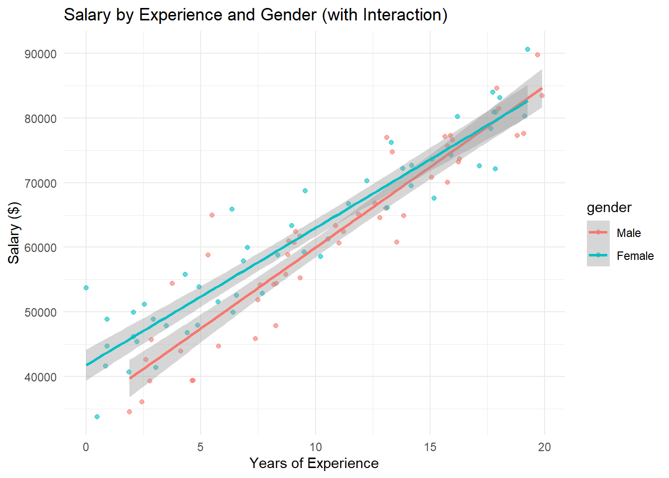
# Extract slopes for each group
coef(model)["experience"]  # Slope for males (reference)
experience
2500.915 coef(model)["experience"] + coef(model)["experience:genderFemale"] # Slope for femalesexperience
2124.041 4.9.1 Key Takeaways
- Interactions allow effects to vary: The impact of one variable depends on another variable’s value
- Parallel slopes assumption: No interaction means equal slopes across groups
- Interpretation changes: With interactions, main effects represent conditional effects
- Visualization helps: Plotting interaction effects aids interpretation and communication
4.9.2 Common Pitfalls
- Centering continuous variables: Consider mean-centering for easier interpretation of main effects
- Higher-order terms: Three-way interactions and beyond become very difficult to interpret
- Sample size: Interactions require larger samples to detect reliably
- Multiple comparisons: Be cautious when testing many potential interactions
4.9.3 Confidence Intervals for Coefficients
We can likewise get confidence intervals for the coefficients. They take the general form:
\[\hat \beta_i \pm t_{\alpha/2, df} \cdot SE_{\hat \beta_i}\]
Again the \(t_{\alpha/2}\) quantile depends on the value for \(\alpha\) of the desired nominal confidence level \(1 - \alpha\).
To get the confidence intervals we use the confint() function just before.
confint(riskLm, level = 0.99) 0.5 % 99.5 %
(Intercept) -0.4730459 2.08402798
stayLength 0.1379482 0.41299604
cultureRatio 0.0307672 0.08213574The estimated change in the mean of infectionRisk is:
- From 0.138 to 0.413 at 99% confidence when increasing
stayLengthby 1 day. (And keepingcultureRatioconstant.) - From 0.031 to 0.082 at 99% confidence when increasing
cultureRatioby 1 (ratios don’t really have units). (KeepingstayLengthconstant.)
4.10 Estimating the Mean/Predicting Future Observations
Getting predictions is similar to before. You use the predict() function, and you need to specify what values you want predictions for.
You make a data.frame with values for each predictor variable.
- You must specify all variables that are used as predictors.
- Each variable must have the same number of points.
- If you screw this up, you will get predictions for all of the original points in the data.
Lets say you want to predict/estimate infectionRisk for a hospital that have an average length of stay of 5, 10, and 15 days, and a average culture ratio of 5, 15, 25. But which way are we combining those?
newdata <- data.frame(stayLength = c(5, 10, 15),
                      cultureRatio = c(5, 15, 25))
predict(riskLm, newdata)
1 2 3
2.465109 4.406984 6.348859 Or what about?
newdata <- data.frame(stayLength = c(5, 10, 15),
                      cultureRatio = c(25, 15, 5))
predict(riskLm, newdata)
1 2 3
3.594138 4.406984 5.219830 Or…?
newdata <- data.frame(stayLength = c(15, 5, 10),
                      cultureRatio = c(15, 25, 5))
predict(riskLm, newdata)
1 2 3
5.784345 3.594138 3.842469 You have to know which exact combination of predictor variable values you want.
4.10.1 Confidence Intervals for the Mean and Prediction Intervals for Future Observations
This is the same as well.
- Confidence intervals (CIs) are establishing a range of plausible values for the conditional mean: \(\mu_{y|x} = \beta_0 + \beta_1 x_1 + \widehat \beta_{2} x_2\)
- Prediction intervals (PIs) establish a range of plausible values for individual observations: \(y = \beta_0 + \beta_1 x_1 + \widehat \beta_{2} x_2 + \epsilon\)
Let’s make 99% CIs and PIs.
newdata <- data.frame(stayLength = c(15, 5, 10),
                      cultureRatio = c(15, 25, 5))
CIs <- predict(riskLm, newdata,
               interval = "confidence", level = 0.99)
PIs <- predict(riskLm, newdata,
               interval = "prediction", level = 0.99)
CIs fit lwr upr
1 5.784345 5.001363 6.567327
2 3.594138 2.803874 4.384403
3 3.842469 3.456304 4.228635PIs fit lwr upr
1 5.784345 3.0409109 8.527779
2 3.594138 0.8486173 6.339659
3 3.842469 1.1849346 6.500004Interpretations are now relative to the value of both predictors variables.
CI Interpretation: There is 99% confidence that the mean infection risk of hospitals with average length of stay of 15 days and culture ratio of 15 is between 5.00% to 6.57%.
PI Interpretation: There is 99% confidence that the infection risk of an Individual hospital with average length of stay of 15 days and culture ratio of 15 is between 3.04% to 8.53%.
4.11 Residual Analysis
To assess validity of the model assumptions we can examine the residuals in the same manner as before. Create plots of the residuals using autoplot() and assess them in the same way as before.
autoplot(riskLm)
4.12 Adding more variables!
The linear model is not restricted to one or two variables. We can have as many predictor variables as we want! Let \(p\) denote the total number of predictor variables we use. The linear model is now:
\[y = \widehat \beta_0 + \widehat \beta_1 x_1 + \widehat \beta_{2} x_2 + ... + \widehat \beta_{p} + \epsilon = \beta_0 + \sum_{k=1}^p\beta_k x_k + \epsilon\]
4.12.1 facilities and infectionRisk?
Here is a graph between facilities and infectionRisk.
ggplot(senic, aes(x = facilities, y = infectionRisk)) +
  geom_point()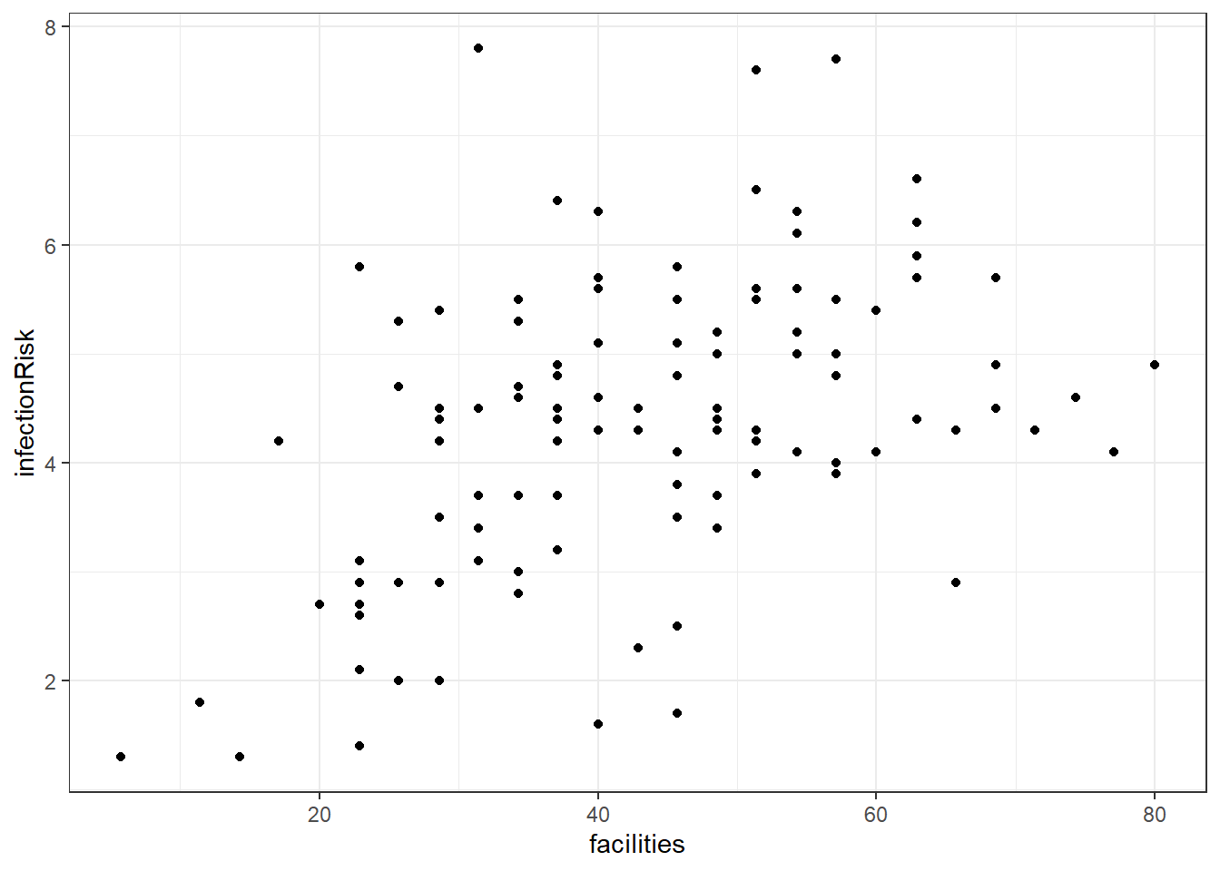
4.12.2 Adding facilities to the infectionRisk model.
riskierLm <- lm(infectionRisk ~ stayLength + cultureRatio + facilities, senic)
summary(riskierLm)
Call:
lm(formula = infectionRisk ~ stayLength + cultureRatio + facilities,
    data = senic)

Residuals:
     Min       1Q   Median       3Q      Max
-2.26400 -0.59873  0.01723  0.56650  2.64517

Coefficients:
             Estimate Std. Error t value Pr(>|t|)
(Intercept)  0.491332   0.481636   1.020  0.30992
stayLength   0.223907   0.053366   4.196 5.56e-05 ***
cultureRatio 0.054200   0.009479   5.718 9.55e-08 ***
facilities   0.019630   0.006454   3.042  0.00295 **
---
Signif. codes:  0 '***' 0.001 '**' 0.01 '*' 0.05 '.' 0.1 ' ' 1

Residual standard error: 0.9674 on 109 degrees of freedom
Multiple R-squared:  0.4934,    Adjusted R-squared:  0.4795
F-statistic: 35.39 on 3 and 109 DF,  p-value: 4.769e-16
4.12.3 Remember to always check your residuals!
autoplot(riskierLm)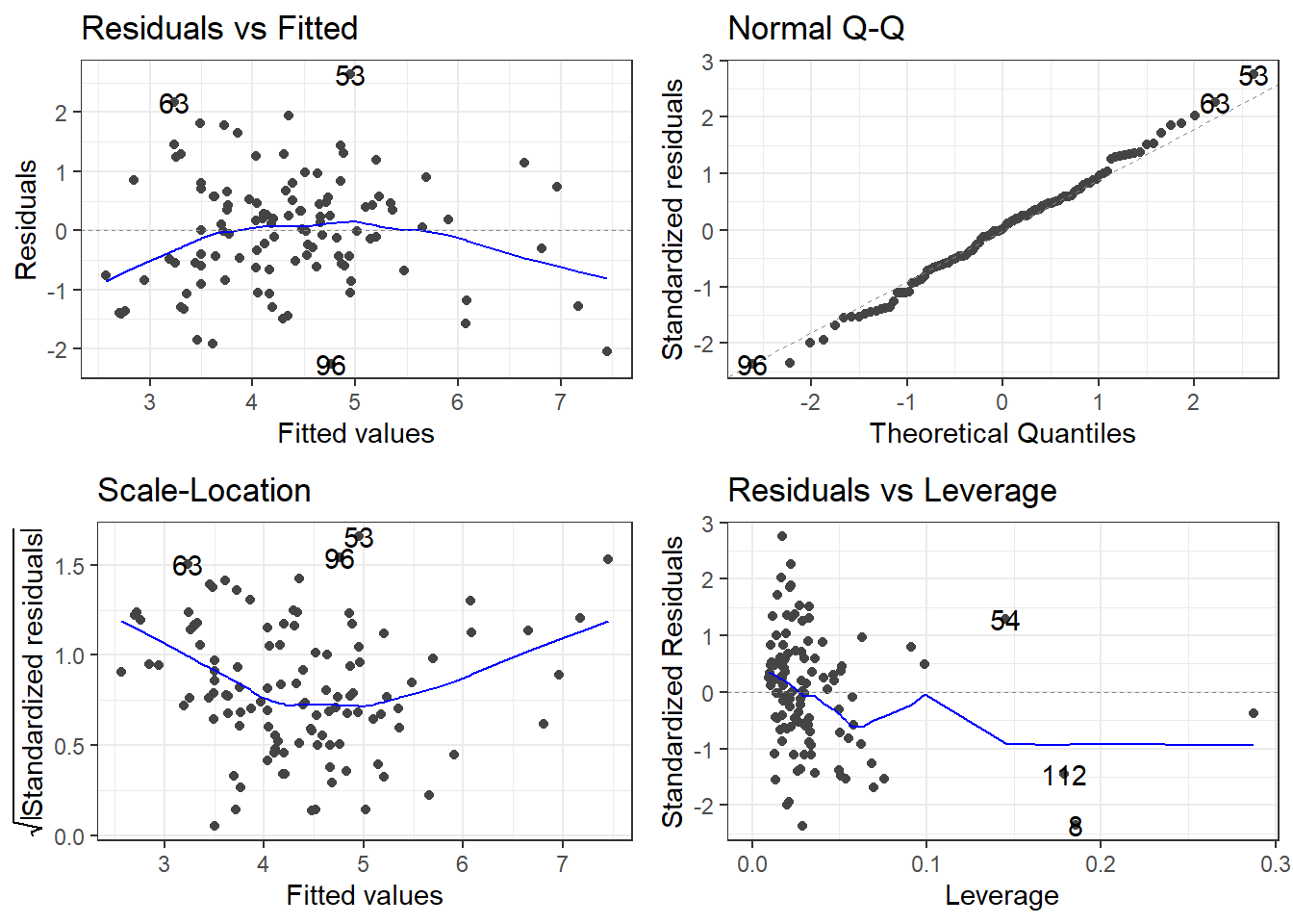
4.12.4 The Model Analysis of Variance: Global F-Test
Assuming there are \(p\) predictor variables
\(H_0: \beta_1 = \beta_2 = \dots = \beta_p = 0\)
\(H_1:\) At least one \(\beta_k\) is not \(0\).
To test this, we use that same breakdown of model variability as before:
\[SSTO = \sum_{i=1}^n(y_i - \bar y)^2\]
This variability in the variable can be broken up into two pieces:
\[SSR = \sum_{i=1}^n(\hat y_i - \bar y)^2 = \sum_{i=1}^n(\widehat \mu_{y|x} - \widehat\mu_y)^2\]
\[SSE = \sum_{i=1}^n(y_i - \widehat y_i)^2\]
The two sums of squares combined are the total variability \(SSTO\).
\[SSTO = SSR + SSE\] The Regression Degrees of Freedom is now \(p\), the error degrees of freedom is \(n - (p + 1)\).
This gives the following mean squares
- Mean Square Regression: \(MSR = SSR/p\)
- Mean Square Error: \(MSE = SSE/[n-(p+1)]\)
The test statistic is \(F_t = MSR/MSE\) and we use the \(F(p, n-(p +1))\) distribution to compute the p-value.
\[ F_t = \frac{SSR \div p}{MSE} = \frac{MSR}{MSE} \]
4.12.5 F-Test for infectionRisk model with 3 predictors
This test is available via the model summary in the very last row.
summary(riskierLm)
Call:
lm(formula = infectionRisk ~ stayLength + cultureRatio + facilities,
    data = senic)

Residuals:
     Min       1Q   Median       3Q      Max
-2.26400 -0.59873  0.01723  0.56650  2.64517

Coefficients:
             Estimate Std. Error t value Pr(>|t|)
(Intercept)  0.491332   0.481636   1.020  0.30992
stayLength   0.223907   0.053366   4.196 5.56e-05 ***
cultureRatio 0.054200   0.009479   5.718 9.55e-08 ***
facilities   0.019630   0.006454   3.042  0.00295 **
---
Signif. codes:  0 '***' 0.001 '**' 0.01 '*' 0.05 '.' 0.1 ' ' 1

Residual standard error: 0.9674 on 109 degrees of freedom
Multiple R-squared:  0.4934,    Adjusted R-squared:  0.4795
F-statistic: 35.39 on 3 and 109 DF,  p-value: 4.769e-16
Does this really matter? Ask yourself what the null hypothesis would and if it would matter.
4.12.6 Experiment: What happens to the stayLength slope?
Let’s look at the coefficients for the three models involving stayLength as a predictor.
By itself.
| term | estimate | std.error | statistic | p.value |
|---|---|---|---|---|
| (Intercept) | 0.7443037 | 0.5538573 | 1.343855 | 0.1817359 |
| stayLength | 0.3742169 | 0.0563195 | 6.644530 | 0.0000000 |
With cultureRatio.
coeff.summary(riskLm)| term | estimate | std.error | statistic | p.value |
|---|---|---|---|---|
| (Intercept) | 0.8054910 | 0.4877558 | 1.651423 | 0.1015044 |
| stayLength | 0.2754721 | 0.0524647 | 5.250615 | 0.0000007 |
| cultureRatio | 0.0564515 | 0.0097984 | 5.761279 | 0.0000001 |
And finally adding in facilities.
coeff.summary(riskierLm)| term | estimate | std.error | statistic | p.value |
|---|---|---|---|---|
| (Intercept) | 0.4913323 | 0.4816361 | 1.020132 | 0.3099249 |
| stayLength | 0.2239075 | 0.0533656 | 4.195726 | 0.0000556 |
| cultureRatio | 0.0542000 | 0.0094793 | 5.717698 | 0.0000001 |
| facilities | 0.0196303 | 0.0064539 | 3.041603 | 0.0029482 |
4.13 Transformations
A simple way to check the relationship between the variables would be to use the pairs() function. The pairs() function produces scatterplots between all variables you specify.
The basic syntax is pairs(formula, data) where formula is the formula of the regression model you are considering data is the dataset you are using.
pairs(infectionRisk ~ stayLength + cultureRatio + facilities,
      senic)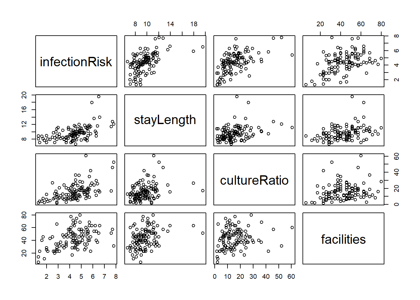
This is a scatterplot matrix. Notice that the vertical axis determined by the variable named to the left or right of a plot, and horizontal axis is determined by the variable named above or below a plot.
4.13.1 Finding the right transformations
pairs(infectionRisk ~ log(stayLength) +
        log(cultureRatio) +
        facilities, senic)
4.13.2 Incorporating them into the model
friskyLm <- lm(infectionRisk ~ log(stayLength) +
                 log(cultureRatio) +
                 facilities, senic)
summary(friskyLm)
Call:
lm(formula = infectionRisk ~ log(stayLength) + log(cultureRatio) +
    facilities, data = senic)

Residuals:
     Min       1Q   Median       3Q      Max
-2.31059 -0.63488  0.04808  0.54228  2.43225

Coefficients:
                   Estimate Std. Error t value Pr(>|t|)
(Intercept)       -4.255154   1.110040  -3.833 0.000212 ***
log(stayLength)    2.534644   0.540984   4.685 8.12e-06 ***
log(cultureRatio)  0.924657   0.134138   6.893 3.70e-10 ***
facilities         0.012736   0.006254   2.036 0.044147 *
---
Signif. codes:  0 '***' 0.001 '**' 0.01 '*' 0.05 '.' 0.1 ' ' 1

Residual standard error: 0.9138 on 109 degrees of freedom
Multiple R-squared:  0.548, Adjusted R-squared:  0.5355
F-statistic: 44.05 on 3 and 109 DF,  p-value: < 2.2e-16
4.13.3 Residuals!
autoplot(friskyLm)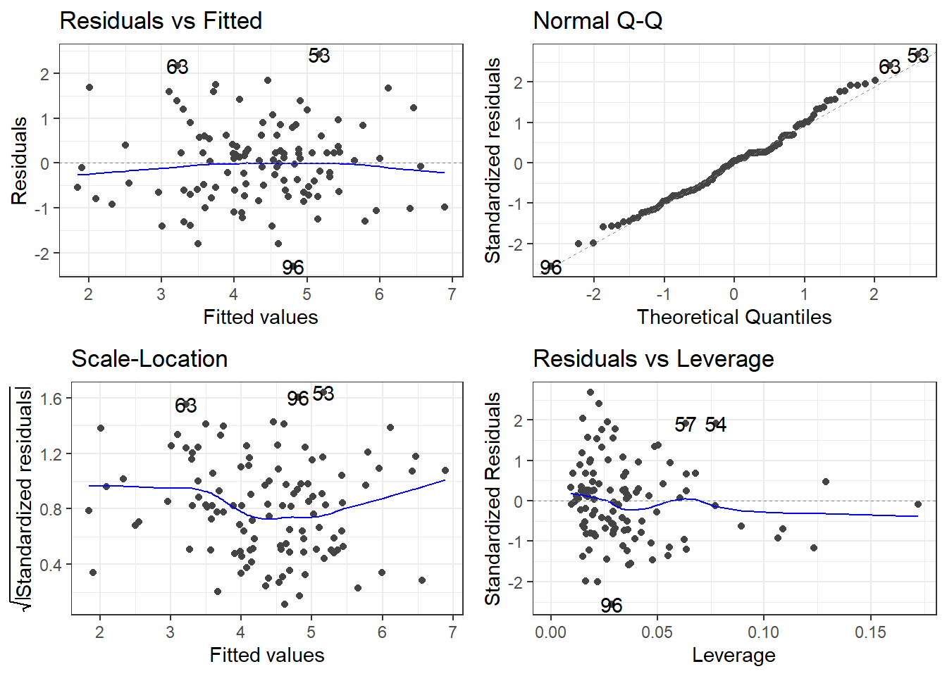
Then you have to reinterpret everything, and so on and so on.
4.13.4 Which log?
friskyLm2 <- lm(infectionRisk ~ log2(stayLength) +
                  log2(cultureRatio) +
                  facilities, senic)
summary(friskyLm2)
Call:
lm(formula = infectionRisk ~ log2(stayLength) + log2(cultureRatio) +
    facilities, data = senic)

Residuals:
     Min       1Q   Median       3Q      Max
-2.31059 -0.63488  0.04808  0.54228  2.43225

Coefficients:
                    Estimate Std. Error t value Pr(>|t|)
(Intercept)        -4.255154   1.110040  -3.833 0.000212 ***
log2(stayLength)    1.756881   0.374982   4.685 8.12e-06 ***
log2(cultureRatio)  0.640923   0.092977   6.893 3.70e-10 ***
facilities          0.012736   0.006254   2.036 0.044147 *
---
Signif. codes:  0 '***' 0.001 '**' 0.01 '*' 0.05 '.' 0.1 ' ' 1

Residual standard error: 0.9138 on 109 degrees of freedom
Multiple R-squared:  0.548, Adjusted R-squared:  0.5355
F-statistic: 44.05 on 3 and 109 DF,  p-value: < 2.2e-16
4.13.5 Can you spot the difference in residuals?
autoplot(friskyLm2)
autoplot(friskyLm)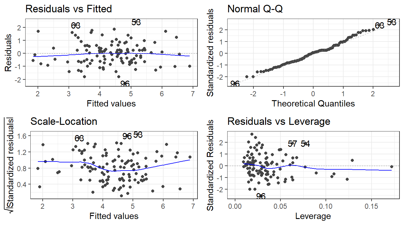
4.14 Variable Selection, Data Reduction, and Model Comparison
4.15 Explainable statistical learning in public health for policy development: the case of real-world suicide data
We will work with data made available from this paper:
https://bmcmedresmethodol.biomedcentral.com/articles/10.1186/s12874-019-0796-7
If you want to go really in-depth of how you deal with data, this article goes into a lot of detail.
phe <- read_csv(here::here("datasets","phe.csv"))4.15.1 Variables. A LOT!
| Variables |
|---|
| 2014 Suicide (age-standardised rate per 100,000 - outcome measure) |
| 2013 Adult social care users who have as much social contact as they would like (% of adult social care users) |
| 2013 Adults in treatment at specialist alcohol misuse services (rate per 1000 population) |
| 2013 Adults in treatment at specialist drug misuse services (rate per 1000 population) |
| 2013 Alcohol-related hospital admission (female) (directly standardised rate per 100,000 female population) |
| 2013 Alcohol-related hospital admission (male) (directly standardised rate per 100,000 male population) |
| 2013 Alcohol-related hospital admission (directly standardised rate per 100,000 population) |
| 2013 Children in the youth justice system (rate per 1,000 aged 10–18) |
| 2013 Children leaving care (rate per 10,000 < 18 population) |
| 2013 Depression recorded prevalence (% of adults with a new diagnosis of depression who had a bio-psychosocial assessment) |
| 2013 Domestic abuse incidents (rate per 1,000 population) |
| 2013 Emergency hospital admissions for intentional self-harm (female) (directly age-standardised rate per 100,000 women) |
| 2013 Emergency hospital admissions for intentional self-harm (male) (directly age-standardised rate per 100,000 men) |
| 2013 Emergency hospital admissions for intentional self-harm (directly age-and-sex-standardised rate per 100,000) |
| 2013 Looked after children (rate per 10,000 < 18 population) |
| 2013 Self-reported well-being - high anxiety (% of people) |
| 2013 Severe mental illness recorded prevalence (% of practice register [all ages]) |
| 2013 Social care mental health clients receiving services (rate per 100,000 population) |
| 2013 Statutory homelessness (rate per 1000 households) |
| 2013 Successful completion of alcohol treatment (% who do not represent within 6 months) |
| 2013 Successful completion of drug treatment - non-opiate users (% who do not represent within 6 months) |
| 2013 Successful completion of drug treatment - opiate users (% who do not represent within 6 months) |
| 2013 Unemployment (% of working-age population) |
| 2012 Adult carers who have as much social contact as they would like (18+ yrs) (% of 18+ carers) |
| 2012 Adult carers who have as much social contact as they would like (all ages) (% of adult carers) |
| 2011 Estimated prevalence of opiates and/or crack cocaine use (rate per 1,000 aged 15–64) |
| 2011 Long-term health problems or disability (% of people whose day-to-day activities are limited by their health or disability) |
| 2011 Marital breakup (% of adults whose current marital status is separated or divorced) |
| 2011 Older people living alone (% of households occupied by a single person aged 65 or over) |
| 2011 People living alone (% of all households occupied by a single person) |
| Mental Health Service users with crisis plans: % of people in contact with services with a crisis plan in place (end of quarter snapshot) |
| Older people |
| 2011 Self-reported well-being - low happiness (% of people with a low happiness score) |
4.16 How do we choose variables?
Objective: Find a way to predict suicide rates.
We could just use all of the predictors in a linear model.
fullLm <- lm(suicide_rate ~ ., phe)

summary(fullLm)
Call:
lm(formula = suicide_rate ~ ., data = phe)

Residuals:
    Min      1Q  Median      3Q     Max
-3.0118 -1.0447 -0.2702  0.9903  4.1993

Coefficients:
                                 Estimate Std. Error t value Pr(>|t|)
(Intercept)                     2.0155877  3.5059381   0.575    0.566
children_youth_justice         -0.0235629  0.0247292  -0.953    0.343
adult_carers_isolated_18        0.0336685  0.0262501   1.283    0.202
adult_carers_isolated_all_ages -0.0226404  0.0424220  -0.534    0.595
adult_carers_not_isolated       0.3786174  0.2379446   1.591    0.114
alcohol_rx_18                  -0.3001189  0.2515821  -1.193    0.235
alcohol_rx_all_ages            -0.0130574  0.0148093  -0.882    0.380
alcohol_admissions_f           -0.0060296  0.0127911  -0.471    0.638
alchol_admissions_m             0.0167345  0.0268020   0.624    0.534
alcohol_admissions_p           -0.0600782  0.0895445  -0.671    0.504
children_leaving_care           0.0216349  0.0288644   0.750    0.455
depression                     -0.1169805  0.1328876  -0.880    0.380
domestic_abuse                  0.0269278  0.0419236   0.642    0.522
self_harm_female                0.0369915  0.0946913   0.391    0.697
self_harm_male                  0.0318458  0.0944774   0.337    0.737
self_harm_persons              -0.0658812  0.1902674  -0.346    0.730
opiates                         0.2041520  0.1375203   1.485    0.140
lt_health_problems              0.0318830  0.1456081   0.219    0.827
lt_unepmloyment                -0.6342130  1.2588572  -0.504    0.615
looked_after_children           0.0174365  0.0146237   1.192    0.236
marital_breakup                 0.1606036  0.1723378   0.932    0.353
old_pople_alone                 0.3779967  0.4371635   0.865    0.389
alone                          -0.1004305  0.1386281  -0.724    0.470
self_reported_well_being        0.0605038  0.0681410   0.888    0.376
smi                             2.1708482  1.3401643   1.620    0.108
social_care_mh                  0.0006815  0.0005270   1.293    0.199
homeless                       -0.1550536  0.1051424  -1.475    0.143
alcohol_rx                      0.0170587  0.0282631   0.604    0.547
drug_rx_non_opiate             -0.0408008  0.0271119  -1.505    0.135
drug_rx_opiate                  0.1068925  0.0848400   1.260    0.210
unemployment                    0.0690206  0.2925910   0.236    0.814

Residual standard error: 1.687 on 118 degrees of freedom
Multiple R-squared:  0.5031,    Adjusted R-squared:  0.3767
F-statistic: 3.982 on 30 and 118 DF, p-value: 3.823e-08autoplot(fullLm)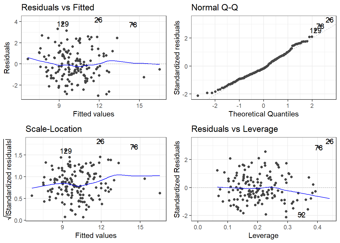
If we are going by statistical significance, each predictor variable fails but the global F-test says that a linear model is working (sort of).
And that \(R^2\) is pretty good for “prediciting” something related to human behavior.
Residuals look good.
Overall, this is bad!
You do not just use all the variables you have
Though there are exceptions: read Harrell’s Regression Model Strategies (Chapter 4, Section 12, 4.12.1 - 4.12.3)
4.16.1 The scope of the problem
How many variables are there to use…? How well do they work?
We could try cor(phe) and see which variables are most correlated with suicide_rate. (You’ll get a lot of output… that’s \(31\times 31 = 961\) correlations)
I’ll save you the pain and just show the correlations with just suicide_rate.
                               suicide_rate
children_youth_justice           0.05847330
adult_carers_isolated_18         0.24939518
adult_carers_isolated_all_ages   0.20369843
adult_carers_not_isolated        0.45228878
alcohol_rx_18                    0.38997284
alcohol_rx_all_ages              0.33117982
alcohol_admissions_f             0.29906808
alchol_admissions_m              0.31868168
alcohol_admissions_p             0.11433511
children_leaving_care            0.36700280
depression                       0.32509700
domestic_abuse                   0.14835220
self_harm_female                 0.49025136
self_harm_male                   0.52004798
self_harm_persons                0.51686092
opiates                          0.41195709
lt_health_problems               0.47825399
lt_unepmloyment                  0.19643927
looked_after_children            0.51243274
marital_breakup                  0.39971208
old_pople_alone                  0.39870200
alone                            0.31037882
self_reported_well_being         0.12949288
smi                              0.18390513
social_care_mh                   0.20125278
homeless                        -0.32105739
alcohol_rx                      -0.07513134
drug_rx_non_opiate              -0.14207504
drug_rx_opiate                  -0.14345307
unemployment                     0.18827138
4.16.2 Just use the best correlations?
These are a few of the strongest correlations.
                               suicide_rate

self_harm_female                 0.49025136
self_harm_male                   0.52004798
self_harm_persons                0.51686092
looked_after_children            0.51243274
Let’s make a model.
badIdea <- lm(suicide_rate ~ self_harm_female + self_harm_male + self_harm_persons + looked_after_children, phe)

summary(badIdea)
Call:
lm(formula = suicide_rate ~ self_harm_female + self_harm_male +
    self_harm_persons + looked_after_children, data = phe)

Residuals:
    Min      1Q  Median      3Q     Max
-4.1974 -1.2196  0.0677  1.1319  6.4354

Coefficients:
                       Estimate Std. Error t value Pr(>|t|)
(Intercept)            6.521275   0.485989  13.419  < 2e-16 ***
self_harm_female       0.059297   0.087465   0.678 0.498889
self_harm_male         0.053601   0.087682   0.611 0.541954
self_harm_persons     -0.106747   0.175961  -0.607 0.545038
looked_after_children  0.031342   0.008442   3.713 0.000292 ***
---
Signif. codes:  0 '***' 0.001 '**' 0.01 '*' 0.05 '.' 0.1 ' ' 1

Residual standard error: 1.763 on 144 degrees of freedom
Multiple R-squared:  0.3379,    Adjusted R-squared:  0.3195
F-statistic: 18.37 on 4 and 144 DF,  p-value: 3.246e-12
What does the model have to say about how the self harm variables are related to suicide rate?
4.17 Multicollinearity
pairs(suicide_rate ~ self_harm_persons + self_harm_female + self_harm_male, phe)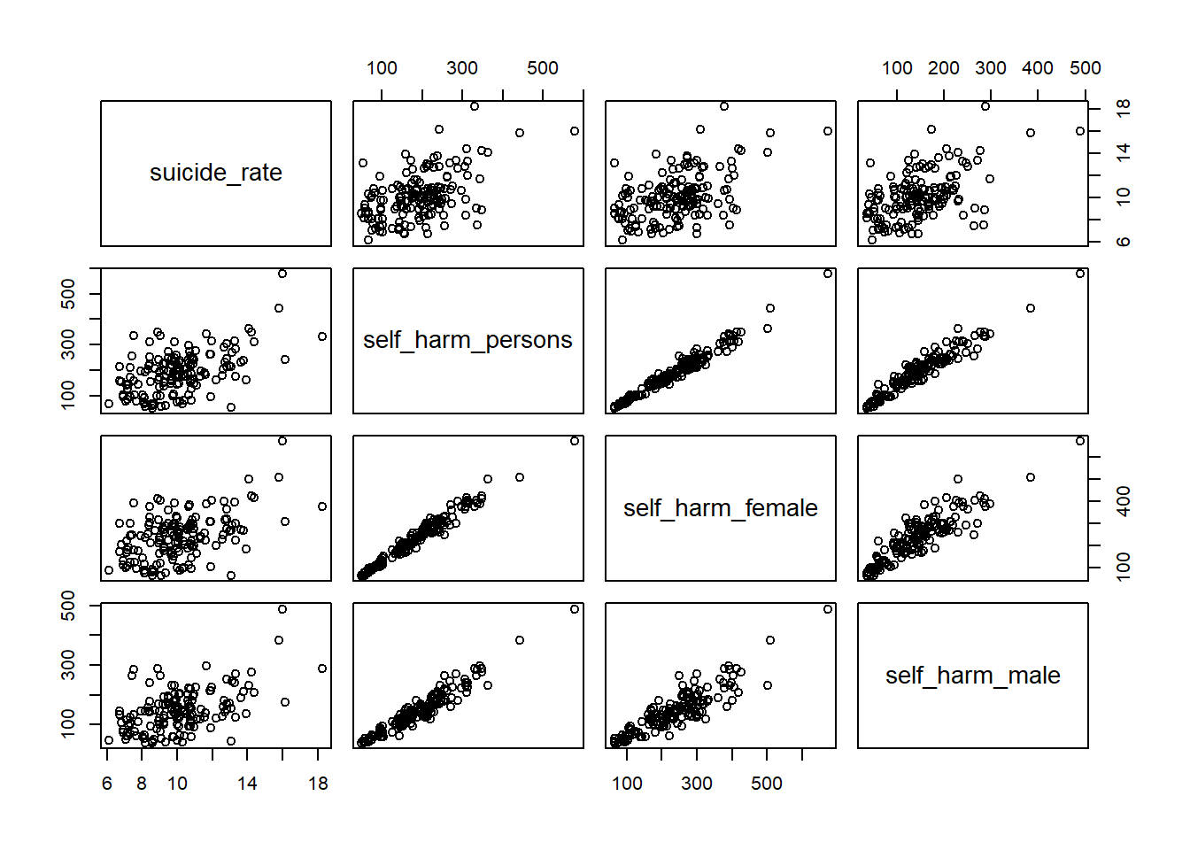
cor(phe$self_harm_female,phe$self_harm_male)[1] 0.8865727cor(phe$self_harm_persons,phe$self_harm_male)[1] 0.9601094cor(phe$self_harm_persons,phe$self_harm_female)[1] 0.9804772When we have predictor variables that are linearly related to each other, we have what is called multi-collinearity.
These variables essentially all contribute the same information over and over to the model. This makes a feedback loop that kicks everything around.
What about a model with just self_harm_persons (Why that one?) and looked_after_children?
notAsBadLm <- lm(suicide_rate ~ self_harm_persons + looked_after_children, phe)

summary(notAsBadLm)
Call:
lm(formula = suicide_rate ~ self_harm_persons + looked_after_children,
    data = phe)

Residuals:
    Min      1Q  Median      3Q     Max
-4.3450 -1.2323  0.0677  1.0792  6.2763

Coefficients:
                      Estimate Std. Error t value Pr(>|t|)
(Intercept)           6.704515   0.430054  15.590  < 2e-16 ***
self_harm_persons     0.008385   0.002124   3.947 0.000123 ***
looked_after_children 0.027803   0.007281   3.818 0.000198 ***
---
Signif. codes:  0 '***' 0.001 '**' 0.01 '*' 0.05 '.' 0.1 ' ' 1

Residual standard error: 1.756 on 146 degrees of freedom
Multiple R-squared:  0.3337,    Adjusted R-squared:  0.3246
F-statistic: 36.56 on 2 and 146 DF,  p-value: 1.344e-13
4.17.1 But what about self harm and looking after children?
Relations may not be as blaringly obvious as that. What about self harm and looking after children?
ggplot(phe, aes(x = self_harm_persons, y = looked_after_children)) +
  geom_point() +
  stat_cor()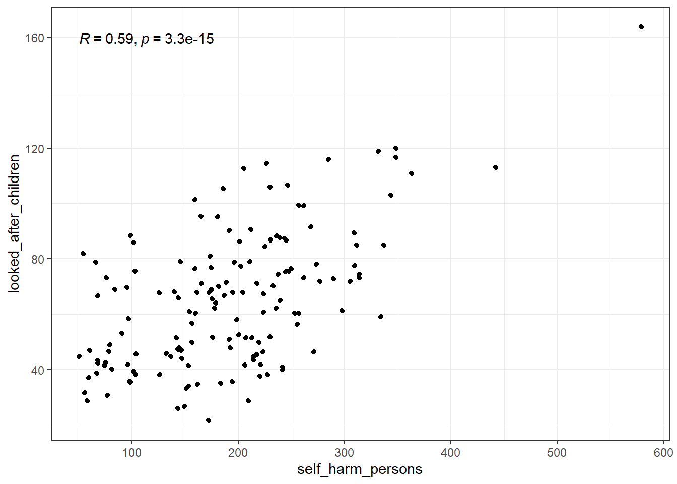
This isn’t nearly as bad and wouldn’t be considered a detrimental relation.
4.18 Measuring multi-collinearity
4.18.1 A linear model for the predictors
Linear relation between many predictor variables.
\[x_k =\beta_{0}^* + \beta_{1}^* x_1 + \beta_{2}^*x_2 + \dots + \beta_p^* x_p + \epsilon^*\]
This is like any model and has it’s own \(R^2\) \(R^2_k\).
If this \(R^2\) is high, it means that a predictor variable is redundant.
There are a few ways to measure “high”.
Some sources would say that \(0.8 \le R_k^2 \le 0.9\) would be problematic, and you have extreme multicollinearity issues for anything higher.
4.18.2 Tolerance
Tolerance is \(1 - R^2_k\).
That’s it.
So \(0.2\) is the “problematic” cutoff and \(0.9\) is the “extreme” cutoff.
It may be referred to as TOL sometimes.
4.18.3 Variance Inflation Factors
The Variance Inflation Factor is:
\[VIF_k = \frac{1}{1 - R^2_k}\]
The VIF is considered “problematic” if greater than 5, and “extreme” if greater than 10.
4.18.4 Getting TOL or VIF: performance package
A nifty package that will help us deal with all the nasty bits of linear regression in R is the performance package. It is part of the easystats universe of packages.
To get tolerance and VIFs, create the model using lm(), and then plug it into the check_collinearity function.
check_collinearity(model)
library(performance)
library(see)

# badidea was the model with all the self harm variables

check_collinearity(badIdea)
# Check for Multicollinearity
Low Correlation
Term VIF VIF 95% CI adj. VIF Tolerance
looked_after_children 2.04 [ 1.66, 2.63] 1.43 0.49
Tolerance 95% CI
[0.38, 0.60]
High Correlation
Term VIF VIF 95% CI adj. VIF Tolerance
self_harm_female 3811.50 [2809.27, 5171.42] 61.74 2.62e-04
self_harm_male 1863.65 [1373.68, 2528.51] 43.17 5.37e-04
self_harm_persons 10400.43 [7665.39, 14111.48] 101.98 9.61e-05
Tolerance 95% CI
[0.00, 0.00]
[0.00, 0.00]
[0.00, 0.00]Versus
check_collinearity(notAsBadLm)# Check for Multicollinearity
Low Correlation
Term VIF VIF 95% CI adj. VIF Tolerance Tolerance 95% CI
self_harm_persons 1.53 [1.29, 1.96] 1.24 0.65 [0.51, 0.78]
looked_after_children 1.53 [1.29, 1.96] 1.24 0.65 [0.51, 0.78]4.18.5 Plot check_collinearity checks
plot(check_collinearity(badIdea))
Versus
plot(check_collinearity(notAsBadLm))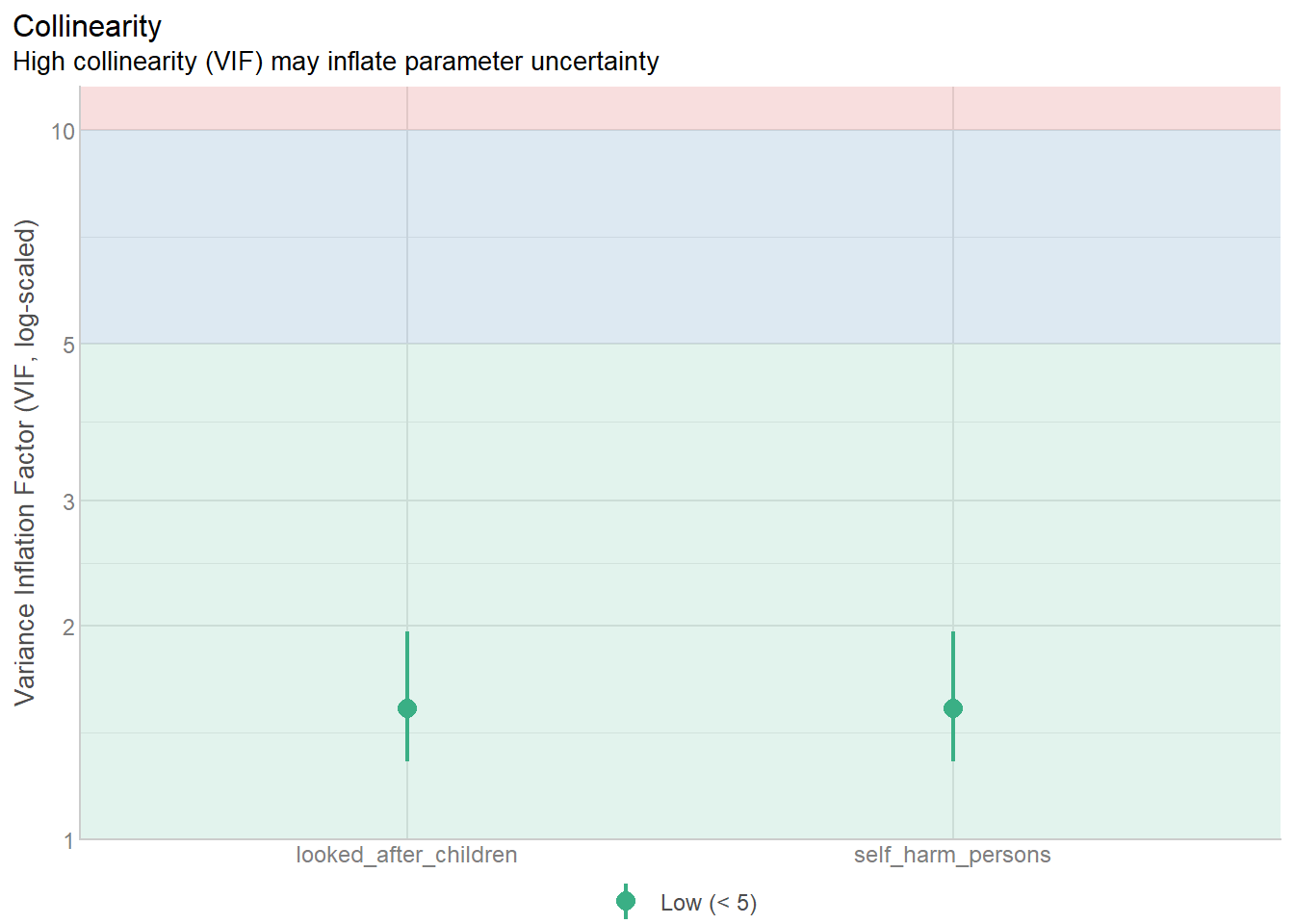
4.18.6 VIF and Tolerance in the full model
You do not get rid of a variable because it has a small tolerance/large VIF!
You would investigate which variables are most correlated with eachother.
You need to use your own reasoning to decide which variables to remove based on the correlations between predictors AND the response.
Tolerance and VIF only indicate that the overall model has a problem, not the individual variable.
check_collinearity(fullLm)# Check for Multicollinearity
Low Correlation
Term VIF VIF 95% CI adj. VIF Tolerance
children_youth_justice 1.48 [ 1.29, 1.80] 1.22 0.68
adult_carers_isolated_18 1.88 [ 1.59, 2.30] 1.37 0.53
adult_carers_isolated_all_ages 1.84 [ 1.57, 2.26] 1.36 0.54
adult_carers_not_isolated 3.11 [ 2.55, 3.88] 1.76 0.32
alcohol_admissions_p 2.05 [ 1.73, 2.52] 1.43 0.49
children_leaving_care 4.32 [ 3.49, 5.42] 2.08 0.23
depression 2.73 [ 2.25, 3.38] 1.65 0.37
domestic_abuse 1.90 [ 1.61, 2.33] 1.38 0.53
marital_breakup 2.36 [ 1.97, 2.91] 1.54 0.42
alone 4.82 [ 3.88, 6.06] 2.19 0.21
self_reported_well_being 1.42 [ 1.24, 1.72] 1.19 0.71
smi 3.62 [ 2.94, 4.52] 1.90 0.28
social_care_mh 1.29 [ 1.15, 1.58] 1.14 0.77
homeless 3.11 [ 2.55, 3.87] 1.76 0.32
alcohol_rx 3.27 [ 2.68, 4.08] 1.81 0.31
drug_rx_non_opiate 3.21 [ 2.63, 4.00] 1.79 0.31
drug_rx_opiate 1.99 [ 1.68, 2.44] 1.41 0.50
Tolerance 95% CI
[0.56, 0.78]
[0.43, 0.63]
[0.44, 0.64]
[0.26, 0.39]
[0.40, 0.58]
[0.18, 0.29]
[0.30, 0.44]
[0.43, 0.62]
[0.34, 0.51]
[0.16, 0.26]
[0.58, 0.81]
[0.22, 0.34]
[0.63, 0.87]
[0.26, 0.39]
[0.24, 0.37]
[0.25, 0.38]
[0.41, 0.60]
Moderate Correlation
Term VIF VIF 95% CI adj. VIF Tolerance
lt_unepmloyment 5.30 [ 4.26, 6.68] 2.30 0.19
looked_after_children 6.68 [ 5.33, 8.45] 2.58 0.15
unemployment 8.68 [ 6.89, 11.02] 2.95 0.12
Tolerance 95% CI
[0.15, 0.23]
[0.12, 0.19]
[0.09, 0.15]
High Correlation
Term VIF VIF 95% CI adj. VIF Tolerance
alcohol_rx_18 18.48 [ 14.52, 23.59] 4.30 0.05
alcohol_rx_all_ages 351.34 [ 273.84, 450.86] 18.74 2.85e-03
alcohol_admissions_f 978.20 [ 762.20, 1255.50] 31.28 1.02e-03
alchol_admissions_m 2345.59 [ 1827.47, 3010.68] 48.43 4.26e-04
self_harm_female 4877.78 [ 3800.20, 6261.00] 69.84 2.05e-04
self_harm_male 2362.51 [ 1840.66, 3032.40] 48.61 4.23e-04
self_harm_persons 13277.66 [10344.20, 17043.10] 115.23 7.53e-05
opiates 12.46 [ 9.83, 15.87] 3.53 0.08
lt_health_problems 11.71 [ 9.25, 14.91] 3.42 0.09
old_pople_alone 11.18 [ 8.84, 14.23] 3.34 0.09
Tolerance 95% CI
[0.04, 0.07]
[0.00, 0.00]
[0.00, 0.00]
[0.00, 0.00]
[0.00, 0.00]
[0.00, 0.00]
[0.00, 0.00]
[0.06, 0.10]
[0.07, 0.11]
[0.07, 0.11]You have to jump through a lot of hoops and then make justifiable choices.
4.18.7 Detecting Multicollinearity
The following our indicators of multicollinearity:
- “Significant” correlations between pairs of independent variables.
- Non-significant t-tests for all or nearly all of the predictor variables, but a significant global F-test.
- The coefficients have opposite signs than what would be expected (by logic or compared to the individual correlation with the response variable).
- A single VIF of 10, more than one VIF of 5 or above. Several VIF 3 or over. Or corresponding tolerance values. Or corresponding \(R^2_k\) values
The cutoffs for VIF, tolerance, or \(R^2_k\) are guidelines not solid rules. Theory should always trump these more arbitrary statistical rules.
4.19 What VIF actually measures
You will read methods sections that say, almost verbatim, “all VIFs were below 10, so multicollinearity was not a concern.” It is worth pausing on what that sentence actually claims, because it usually claims far more than it can support (Kalnins and Praitis Hill 2025).
Everything that follows is organized around a small map. Three different problems travel under the word “collinearity,” and they live on three separate axes:
- Variance. Collinearity inflates the sampling variance of the coefficients. This pushes you toward type 2 error (missing a real effect). VIF is the diagnostic that lives here, and only here.
- Specification bias. Collinearity amplifies the bias from leaving a relevant variable out of the model. This pushes you toward type 1 error (declaring an effect that is an artifact). This is the axis we build up to in Section 4.21.
- Estimator choice. Once variance is high, you may voluntarily trade a little bias for a lot less variance (ridge, subset selection, principal-components regression). The bias here is chosen and in-model, a different animal from axis 2.
The single most common error in applied work is using an axis-1 diagnostic to defend an axis-2 claim. Keep the map in view.
4.19.1 What the formula is
You already have the definition from above. To restate it in the language we will use:
\[\mathrm{VIF}_i = \frac{1}{1 - R_i^2}, \qquad \text{Tolerance}_i = 1 - R_i^2 = \frac{1}{\mathrm{VIF}_i},\]
where \(R_i^2\) is the \(R^2\) from regressing predictor \(x_i\) on all the other predictors. There is an equivalent definition as the \(i\)th diagonal element of the inverted predictor correlation matrix (Marquardt 1970). Notice what is, and is not, in that formula: it uses the predictor matrix \(X\) only. The outcome \(y\) never appears.
4.19.2 What VIF is a multiplier of
VIF earns its name because it is literally the factor by which redundancy inflates the variance of a single coefficient:
\[\mathrm{Var}(\hat\beta_i) = \frac{\sigma^2}{(n-1)\,\mathrm{Var}(x_i)}\,\mathrm{VIF}_i.\]
Note
Redundancy is the cause; variance inflation is the consequence. VIF is not “how correlated are my predictors” in the abstract; it is that redundancy as it propagates into \(\mathrm{Var}(\hat\beta_i)\). A VIF of 9 means the standard error of \(\hat\beta_i\) is \(\sqrt{9} = 3\) times larger than it would be if \(x_i\) were orthogonal to the others.
4.19.3 Within OLS, collinearity is a pure variance phenomenon
This is the line you will hear most often, and it is true: ordinary least squares stays unbiased no matter how high VIF climbs. The estimates are still centered on the right value; they are just noisier. So the honest consequence of high VIF is wide confidence intervals and non-significant \(t\)-tests, i.e. type 2 risk. The estimates are not pulled toward a wrong answer (Kalnins and Praitis Hill 2025).
That sentence is true and routinely misleading, because people hear “collinearity does not bias coefficients” and conclude “collinearity cannot produce a wrong answer.” Those are not the same statement. The unbiasedness holds within the model you fit. It says nothing about the model you should have fit, which is the subject of Section 4.21.
TipWhere the bias–variance tradeoff lives (axis 3)
Bias only enters voluntarily, when you widen the estimator beyond OLS. Ridge regression (Marquardt 1970), subset selection, and principal-components regression all buy lower variance by accepting some estimation bias. That is a deliberate choice you make to tame high VIF. Do not confuse it with the specification bias of Section 4.21, which is imposed on you by what you left out, whether you like it or not.
4.19.4 The thresholds are conventions
The familiar cutoffs (problematic above 5, extreme above 10) have no principled derivation; they are rules of thumb that hardened into rules (O’Brien 2007; Kalnins and Praitis Hill 2025). We already flagged that they are guidelines, not law. The deeper point of the next two sections is that the arbitrariness of the cutoff is not even VIF’s worst problem.
So the boundary of what VIF can tell you is sharp: how redundant is \(x_i\) with the other predictors, as that redundancy inflates its variance estimate — and nothing more.
4.20 The partial and semipartial lens
VIF is not the only quantity built by regressing a predictor on the other predictors. The semipartial (or “part”) correlation comes from the same residualization, and putting the two side by side is what exposes VIF’s blind spot.
4.20.1 Partial vs semipartial
Both start by removing the linear influence of the other predictors:
- The partial correlation residualizes both \(x_i\) and \(y\) on the other predictors, then correlates the leftovers.
- The semipartial correlation residualizes only \(x_i\) on the other predictors, then correlates that leftover with the raw \(y\). Its square is the unique share of variance in \(y\) that \(x_i\) explains beyond the others.
4.20.2 The bridge identity
The residualization that defines VIF and the one that defines the semipartial are the same residualization, which gives a clean link between them:
\[\mathrm{sr}_i = \beta_i^{*}\sqrt{1 - R_i^2} = \frac{\beta_i^{*}}{\sqrt{\mathrm{VIF}_i}}, \qquad \mathrm{sr}_i^2 = R^2_{\text{full}} - R^2_{(-i)},\]
where \(\beta_i^{*}\) is the standardized coefficient and \(R^2_{(-i)}\) is the model fit without \(x_i\).
Tip
Read the first identity aloud: for a fixed standardized coefficient, a higher VIF shrinks the variable’s unique contribution. VIF is, quite literally, a count of how little of \(x_i\) is left once the other predictors have taken their share.
4.20.3 Three jobs, three questions
It helps to keep three questions strictly separate:
| Tool | Question it answers | Where it looks |
|---|---|---|
| VIF / tolerance | How redundant is \(x_i\) with the other predictors? | within \(X\) |
| Semipartial correlation | How much unique predictive value does \(x_i\) add to \(y\) beyond the others? | within the model |
| The Section 4.21 concern | Is \(x_i\)’s estimate contaminated by something outside the model? | uncomputable from the observed data |
The first two are answerable from your data. The third is the one that matters most and the one no statistic on your data can settle.
4.20.4 Reading a small semipartial correlation
A small unique contribution is ambiguous on its own, and VIF disambiguates it:
- sr low + VIF low \(\rightarrow\) a genuinely weak association; an inert predictor.
- sr low + VIF high \(\rightarrow\) the variable may matter, but a collinear partner is absorbing its unique signal. This is redundancy, not irrelevance.
Read jointly, sr and VIF tell you more than either does alone.
# Demo A: low VIF can coexist with a near-zero unique contribution.
# Two near-orthogonal predictors, both barely related to the outcome.
set.seed(2024)
n  <- 800
x1 <- rnorm(n)
x2 <- rnorm(n)                          # near-orthogonal to x1 -> low VIF
y  <- 0.02 * x1 + 0.03 * x2 + rnorm(n)  # both barely related to y

m <- lm(y ~ x1 + x2)

# VIF says "no redundancy" (about 1).
# car::vif() returns the same numbers as performance::check_collinearity().
car::vif(m)
x1 x2
1.001648 1.001648 # Unique contribution, as squared semipartial = R^2 increment from adding x_i.
r2_full <- summary(m)$r.squared
r2_no1 <- summary(lm(y ~ x2))$r.squared
r2_no2 <- summary(lm(y ~ x1))$r.squared
c(sr2_x1 = r2_full - r2_no1, sr2_x2 = r2_full - r2_no2) # about 0: inert sr2_x1 sr2_x2
5.021832e-04 1.652242e-05 VIF reports “no collinearity problem” (both about 1.0) while the squared semipartials are essentially zero. Two different questions: VIF says the predictors are not stepping on each other, and the semipartials say they are not earning their seat in the model. A clean VIF table is not a license to keep variables.
4.20.6 A warning for causal work
Important
“This predictor has a small semipartial correlation, so drop it” is a prediction heuristic, and a reasonable one when prediction is the goal. Imported into confounder selection it is dangerous. A confounder need not add much unique predictive value to badly bias a focal coefficient when omitted: its damage runs through its correlation with the included predictors times its effect on \(y\), not through its marginal predictive contribution. Variable selection for prediction and variable selection for causal estimation are different problems with different rules (Greenland et al. 1999; Harrell 2015).
4.21 Bias inflation: the Kalnins critique
We now reach axis 2. The claim of Kalnins and Praitis Hill (2025) is sharp: collinearity’s most serious danger is not the variance inflation that VIF measures, but the way collinearity amplifies omitted-variable bias — and that danger is largest in exactly the situations where VIF looks reassuring.
4.21.1 Omitted-variable bias, briefly
Compare a “long” regression that includes a variable \(Z\) with the “short” regression that omits it. The coefficient on \(X\) in the short regression carries an extra term:
\[\hat\beta^{s}_{X} = \delta^{l}_{X} + \left(\frac{X^{\top}Z}{X^{\top}X}\right)\delta^{l}_{Z},\]
the true effect plus (the regression of the omitted \(Z\) on \(X\)) times (\(Z\)’s effect on \(y\)). The paper works the standardized two-predictor case with an omitted \(Z\), setting the true direct effect to zero (\(\delta^l_X = 0\)) and \(Z\)’s effect to one (\(\delta^l_Z = 1\)), so that every nonzero coefficient you see in the short model is pure bias (Kalnins and Praitis Hill 2025).
4.21.2 The paradox
ImportantConclusion 1: omitting a confounder lowers VIF
Because \(R_i^2\) can only rise as you add predictors, dropping a relevant variable that is correlated with \(x_i\) reduces \(x_i\)’s VIF. The more badly you misspecify the model in this way, the cleaner the VIF table looks. Low VIF and severe bias are not opposites; they routinely occur together.
# Demo B: dropping a confounder lowers VIF while inflating bias.
# A latent confounder Z drives y; x1, x2 are proxies with NO direct effect.
set.seed(11)
n  <- 500
Z  <- rnorm(n)
x1 <- 0.85 * Z + sqrt(1 - 0.85^2) * rnorm(n)   # higher correlation with Z
x2 <- 0.80 * Z + sqrt(1 - 0.80^2) * rnorm(n)   # slightly lower correlation with Z
y  <- 1.0  * Z + rnorm(n)                        # true effects of x1 and x2 are zero

full  <- lm(y ~ x1 + x2 + Z)   # correctly specified: x1, x2 coefficients ~ 0
short <- lm(y ~ x1 + x2)       # confounder Z omitted

# Watch the VIFs FALL when we drop Z (Conclusion 1).
car::vif(full)[c("x1", "x2")]  # higher, because x1, x2, Z are all collinear
x1 x2
3.626181 2.613148 car::vif(short) # lower, after removing the collinear Z x1 x2
1.812655 1.812655 # The short-model coefficients are biased away from their true value of zero,
# and remain comfortably "significant".
summary(short)$coefficients Estimate Std. Error t value Pr(>|t|)
(Intercept) 0.003445162 0.04781672 0.07204932 9.425916e-01
x1 0.563326765 0.06399280 8.80297172 2.216033e-17
x2 0.411452320 0.06523101 6.30761837 6.270067e-10Three things move at once. The VIFs of x1 and x2 fall from roughly 3.6 and 2.6 in the correct model to about 1.8 in the misspecified one. Yet the misspecified coefficients are far from their true value of zero (about 0.56 and 0.41) and both are wildly significant. A reader who trusts the threshold rule, or the \(t\)-statistics, would wave this model through. Only the bias-inflation view explains why it should be distrusted.
4.21.3 Polarization and the observable symptom
A related result is beta polarization (or homogenization): the omitted common factor distorts the coefficients of correlated predictors, with the distortion growing as the correlation \(\theta \to \pm 1\).
Note
In the symmetric proxy setup above, both predictors load positively on \(Z\), so the bias pushes both coefficients the same way (homogenization) rather than flipping a sign. A vivid sign flip needs an asymmetric structure; the clinical example below is the canonical case. The general lesson connects back to Section 4.20: a coefficient whose sign disagrees with its own zero-order correlation with \(y\) is the observable footprint of bias inflation. This is exactly indicator (3) in our earlier multicollinearity checklist.
4.21.4 Bigger samples are not automatically safer
WarningConclusion 5: \(N\) pulls the two axes apart
A larger sample shrinks variance inflation (axis 1 improves), but it raises the type 1 error rate produced by bias inflation (axis 2 worsens). The bias does not average out with more data, because it is not noise; more data just estimates the biased quantity more precisely. This is the result that most surprises statistically trained readers: collecting more data does not rescue a misspecified model, and can make its false conclusions look more authoritative.
4.21.5 A clinical example
Vatcheva et al. (2016) analyze blood pressure with anthropometric predictors. Adding BMI to a model already containing waist circumference flips the waist-circumference coefficient negative and counter-intuitive — implying, absurdly, that a larger waist lowers blood pressure once BMI is held fixed (Kalnins and Praitis Hill 2025). Both the threshold view and the \(t\)-statistic view would pass this model. Only the bias-inflation lens flags it, by noticing the sign flip relative to the zero-order relationship.
4.21.6 What to do instead
VIF cannot be the centerpiece. The defensible workflow leans on judgment and on the outcome, which VIF ignores:
- Inspect the zero-order bivariate correlations among predictors. Treat correlations above about 0.30 as worth scrutiny (about 0.20 once \(N\) is in the thousands).
- Watch for sign flips and implausible magnitudes relative to theory and to prior results.
- Reason about every covariate’s expected sign before fitting, and treat disagreement as a signal to investigate, not a result to report.
- Instrumental variables are the textbook remedy for the omitted-variable problem, with the honest caveat that a weak or invalid instrument can be worse than the disease (Kalnins and Praitis Hill 2025).
- Remember that quadratic terms, interactions, and dummy-coded fixed effects produce large but benign VIFs — one more reason not to lean on the number.
4.21.7 Synthesis
Return to the three-axis map from Section 4.19:
- Variance (VIF): a function of \(X\) alone; high values mean wide intervals and type 2 risk.
- Specification bias (this section): a function of what you left out; invisible to any diagnostic computed from the observed data; the source of type 1 risk.
- Estimator choice: a bias you opt into to tame axis 1, and must keep separate from axis 2.
The error the whole literature keeps making is to take an axis-1 diagnostic and use it to make an axis-2 claim. Said once more, plainly: a diagnostic computed only from your predictors cannot detect a problem that lives in what you left out.
4.22 Variable screening the PHE data
The paper has various methods for variable selection to remove multicollinearity issues.
They don’t really document it that well… Here’s my best take.
# I created this dataset after going through things over and over
# I removed variables from the csv as I was working with it in R
# Lots of fun!

# also, I only use this dataset for demonstration so I don't have to type out
# all of the variables I left in the data into the formula.

pheRed <- read_csv(here::here("datasets",
                              'phe_reduced.csv'))

redModel <- lm(suicide_rate ~ ., pheRed)

check_collinearity(redModel)
# Check for Multicollinearity
Low Correlation
Term VIF VIF 95% CI adj. VIF Tolerance
children_youth_justice 1.13 [1.04, 1.51] 1.06 0.88
adult_carers_isolated_all_ages 1.48 [1.27, 1.85] 1.22 0.68
alcohol_admissions_p 1.78 [1.49, 2.23] 1.33 0.56
children_leaving_care 2.58 [2.09, 3.30] 1.61 0.39
depression 2.21 [1.81, 2.80] 1.49 0.45
domestic_abuse 1.42 [1.23, 1.78] 1.19 0.70
self_harm_persons 2.35 [1.92, 2.99] 1.53 0.43
opiates 2.14 [1.76, 2.70] 1.46 0.47
marital_breakup 1.83 [1.53, 2.30] 1.35 0.55
alone 1.49 [1.28, 1.87] 1.22 0.67
self_reported_well_being 1.24 [1.10, 1.57] 1.11 0.81
social_care_mh 1.17 [1.05, 1.51] 1.08 0.86
homeless 2.25 [1.84, 2.86] 1.50 0.44
alcohol_rx 1.43 [1.24, 1.80] 1.20 0.70
drug_rx_opiate 1.62 [1.37, 2.03] 1.27 0.62
Tolerance 95% CI
[0.66, 0.97]
[0.54, 0.79]
[0.45, 0.67]
[0.30, 0.48]
[0.36, 0.55]
[0.56, 0.81]
[0.33, 0.52]
[0.37, 0.57]
[0.43, 0.65]
[0.54, 0.78]
[0.64, 0.91]
[0.66, 0.95]
[0.35, 0.54]
[0.56, 0.81]
[0.49, 0.73]Some variables I removed because I could not find the correct definition.
I am not an expert on this stuff so I had to do my best based on my mediocre knowledge of the subject matter, and trying to figure out what the authors of the paper were saying.
When it is okay to stop removing variables is entirely dependent on the situation. I don’t even have a guideline for it.
4.23 Next step: Choosing an actual model
Supposing the multicollinearity issue has been solved, how do we move on?
Do we use all the variables in the model?
summary(redModel)
Call:
lm(formula = suicide_rate ~ ., data = pheRed)

Residuals:
    Min      1Q  Median      3Q     Max
-3.8689 -1.1154 -0.0917  0.8901  4.2030

Coefficients:
                                 Estimate Std. Error t value Pr(>|t|)
(Intercept)                     4.0832859  3.0285950   1.348   0.1799
children_youth_justice         -0.0136101  0.0220822  -0.616   0.5387
adult_carers_isolated_all_ages  0.0000509  0.0387482   0.001   0.9990
alcohol_admissions_p           -0.0623441  0.0849678  -0.734   0.4644
children_leaving_care           0.0422261  0.0227752   1.854   0.0659 .
depression                     -0.1622739  0.1220073  -1.330   0.1858
domestic_abuse                  0.0247253  0.0369822   0.669   0.5049
self_harm_persons               0.0066734  0.0025813   2.585   0.0108 *
opiates                         0.1010386  0.0580642   1.740   0.0842 .
marital_breakup                 0.2937180  0.1548091   1.897   0.0600 .
alone                           0.0336382  0.0786620   0.428   0.6696
self_reported_well_being        0.0345748  0.0650050   0.532   0.5957
social_care_mh                  0.0007603  0.0005101   1.490   0.1385
homeless                       -0.2377671  0.0912485  -2.606   0.0102 *
alcohol_rx                     -0.0047326  0.0190770  -0.248   0.8045
drug_rx_opiate                  0.0305590  0.0779842   0.392   0.6958
---
Signif. codes:  0 '***' 0.001 '**' 0.01 '*' 0.05 '.' 0.1 ' ' 1

Residual standard error: 1.72 on 133 degrees of freedom
Multiple R-squared:  0.4176,    Adjusted R-squared:  0.3519
F-statistic: 6.358 on 15 and 133 DF,  p-value: 5.163e-10
Well now at least some of the predictor’s are significant.
We should not just use all predictors since that ruins the generalizibility of the model.
4.23.0.1 The principle of parsimony: Models should have as few variables/parameters as possible while retaining adequacy.
4.24 Methods for model assessment
We have many variables to choose from, and it’s really easy to make a model.
Should we just pick the variables most highly correlated with suicide rate?
What is our cutoff then?
                               suicide_rate
children_youth_justice           0.05847330
adult_carers_isolated_all_ages   0.20369843
alcohol_admissions_p             0.11433511
children_leaving_care            0.36700280
depression                       0.32509700
domestic_abuse                   0.14835220
self_harm_persons                0.51686092
opiates                          0.41195709
marital_breakup                  0.39971208
alone                            0.31037882
self_reported_well_being         0.12949288
social_care_mh                   0.20125278
homeless                        -0.32105739
alcohol_rx                      -0.07513134
drug_rx_opiate                  -0.14345307
cor1 <- lm(suicide_rate ~ self_harm_persons, phe)
cor2 <- lm(suicide_rate ~ self_harm_persons + opiates, phe)
cor3 <- lm(suicide_rate ~ self_harm_persons + opiates + marital_breakup, phe)
cor4 <- lm(suicide_rate ~ self_harm_persons + opiates + marital_breakup +
children_leaving_care, phe)
cor5 <- lm(suicide_rate ~ self_harm_persons + opiates + marital_breakup +
children_leaving_care + depression, phe)
cor6 <- lm(suicide_rate ~ self_harm_persons + opiates + marital_breakup +
children_leaving_care + depression + homeless, phe)- Is the last model the best?
- Should we add more variables?
- Different variables?
4.24.1 Just “significant” variables?
Lets use any of the variables that had a p-value below 0.1.
# Changing model name method since now we will be looking at several models

sig1 <- lm(suicide_rate ~ children_leaving_care + self_harm_persons + opiates + marital_breakup + homeless, phe)

summary(sig1)
Call:
lm(formula = suicide_rate ~ children_leaving_care + self_harm_persons +
    opiates + marital_breakup + homeless, data = phe)

Residuals:
    Min      1Q  Median      3Q     Max
-3.8194 -1.1301 -0.1541  0.9383  5.6420

Coefficients:
                       Estimate Std. Error t value Pr(>|t|)
(Intercept)            4.855937   1.449776   3.349  0.00104 **
children_leaving_care  0.037193   0.019703   1.888  0.06109 .
self_harm_persons      0.005501   0.002307   2.385  0.01840 *
opiates                0.123432   0.050315   2.453  0.01536 *
marital_breakup        0.218171   0.134664   1.620  0.10741
homeless              -0.212926   0.075547  -2.818  0.00551 **
---
Signif. codes:  0 '***' 0.001 '**' 0.01 '*' 0.05 '.' 0.1 ' ' 1

Residual standard error: 1.705 on 143 degrees of freedom
Multiple R-squared:  0.385, Adjusted R-squared:  0.3635
F-statistic: 17.91 on 5 and 143 DF, p-value: 9.201e-14autoplot(sig1)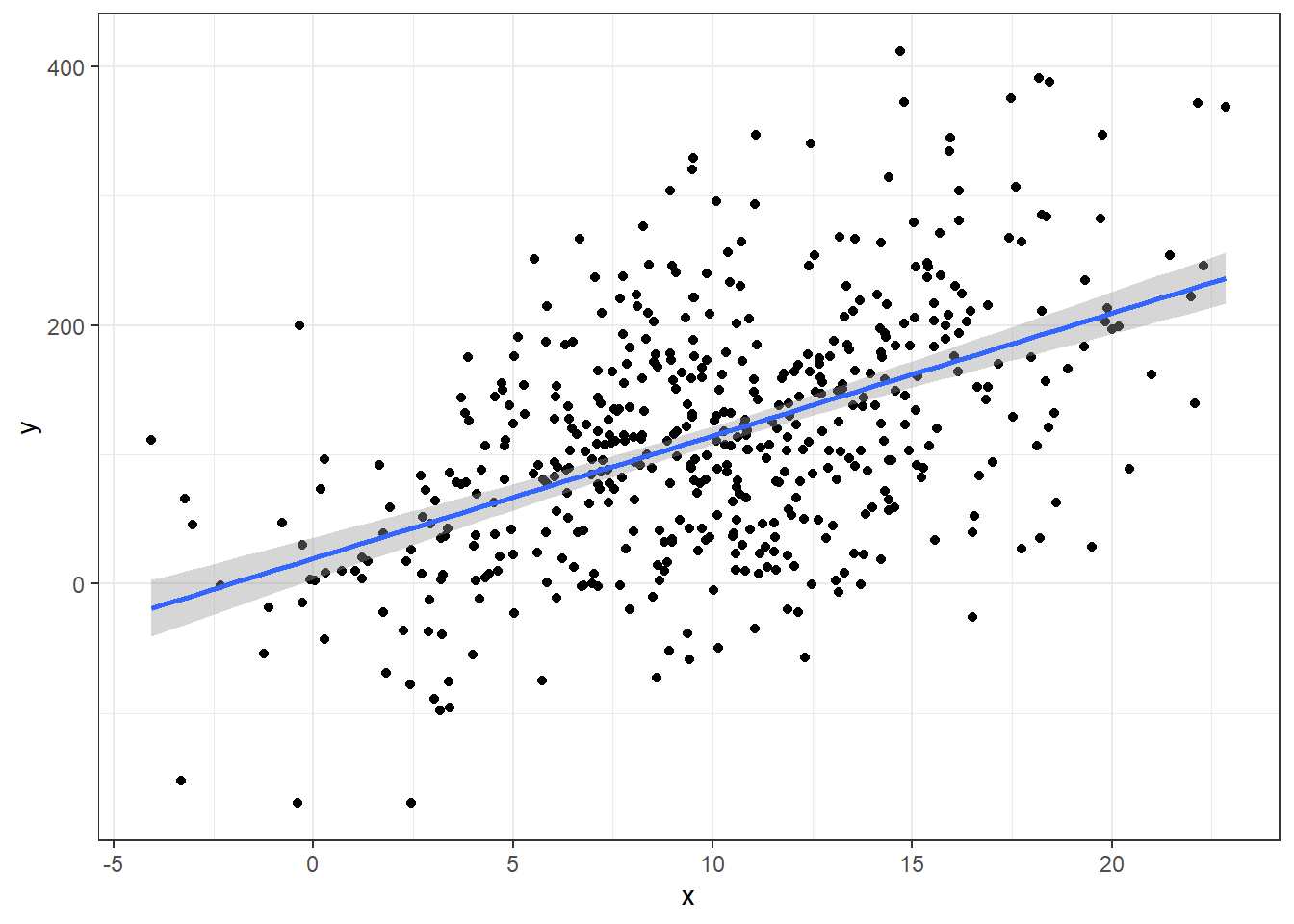
Wait… now marital breakup isn’t significant?
# Changing model name method since now we will be looking at several models

sig2 <- lm(suicide_rate ~ children_leaving_care + self_harm_persons + opiates +
             homeless, phe)

summary(sig2)
Call:
lm(formula = suicide_rate ~ children_leaving_care + self_harm_persons +
    opiates + homeless, data = phe)

Residuals:
    Min      1Q  Median      3Q     Max
-3.8777 -1.1053  0.0011  1.0022  5.8723

Coefficients:
                       Estimate Std. Error t value Pr(>|t|)
(Intercept)            7.033367   0.546679  12.866  < 2e-16 ***
children_leaving_care  0.044142   0.019338   2.283  0.02392 *
self_harm_persons      0.006671   0.002203   3.028  0.00292 **
opiates                0.121234   0.050580   2.397  0.01782 *
homeless              -0.227131   0.075459  -3.010  0.00309 **
---
Signif. codes:  0 '***' 0.001 '**' 0.01 '*' 0.05 '.' 0.1 ' ' 1

Residual standard error: 1.714 on 144 degrees of freedom
Multiple R-squared:  0.3738,    Adjusted R-squared:  0.3564
F-statistic: 21.49 on 4 and 144 DF, p-value: 6.473e-14autoplot(sig2)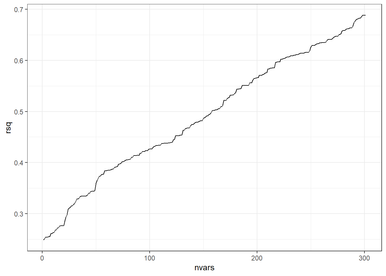
- Relying on “statistical” significance means you will end-up shooting yourself in the foot, metaphorically speaking, i.e., make a bad model.
4.24.2 \(R^2\)? (Don’t use it to choose models).
Recall the definition of \(R^2\): It is the proportion of variability in the response variable explained by your predictor variables in the linear model.
Higher \(R^2\) is better, so maybe we should choose the model with the highest \(R^2\)?
- The full model has an \(R^2\) of 0.5031.
- After whittling down some variables due to multicollinearity,
model1has an \(R^2\) of 0.385. model2has an \(R^2\) of 0.3738.
So the full model is best! Right? All this stuff about variable elimination is pointless. I wasted hours of my life to get to this point…. No!
Never determine which is the best model via \(R^2\).
- \(R^2\) can be arbitrarily high when using many variables that may not be actually related to the response variable in any meaningful way.
n = 500
a = 10; b = 10

### MAKING DATA WITH A TRUE LINEAR MODEL
x <- rnorm(n, 10, 5)
y = a + b*x + rnorm(n,0 ,80)

data <- data.frame(y,x)

ggplot(data, aes(x,y)) +
  geom_point() +
  geom_smooth(method = 'lm')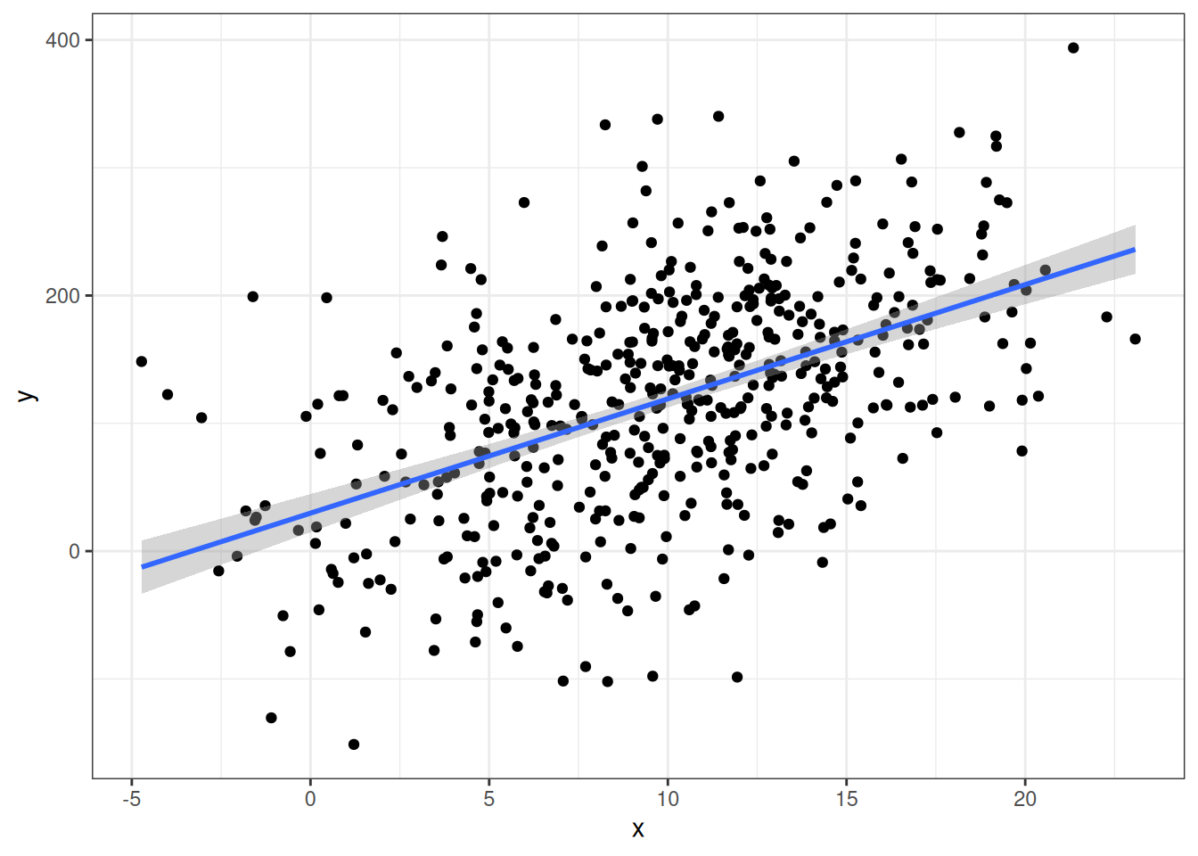
summary(lm(y ~ x, data))
Call:
lm(formula = y ~ x, data = data)

Residuals:
     Min       1Q   Median       3Q      Max
-235.078  -51.081    2.477   52.245  230.116

Coefficients:
            Estimate Std. Error t value Pr(>|t|)
(Intercept)  29.7408     7.6024   3.912 0.000104 ***
x             8.9423     0.6896  12.967  < 2e-16 ***
---
Signif. codes:  0 '***' 0.001 '**' 0.01 '*' 0.05 '.' 0.1 ' ' 1

Residual standard error: 77.25 on 498 degrees of freedom
Multiple R-squared:  0.2524,    Adjusted R-squared:  0.2509
F-statistic: 168.1 on 1 and 498 DF,  p-value: < 2.2e-16
The R-squared here for the perfectly correct model is 0.2524106
- R-squared can be low even when you use the “correct” model.
Now let’s throw in some irrelevant data and graph what happens to R-squared.
# Extra worthless predictors

p = 300

extra.predictors <- data.frame(matrix(rnorm(n*p), nrow=n))

full.data <- data.frame(data, extra.predictors)# need code to combine true and extra data

rsq = rep(NA, p+1)

for(iter in 1:(p+1)){
form <-formula(paste('y ~ ', paste(names(full.data)[2:(iter+1)], collapse=' + ')))
fit.mdl <- lm(form, data=full.data)
rsq[iter] <- summary(fit.mdl)$r.squared # Get the rsq value for the model.
}
ggplot(data.frame(nvars=1:(p+1), rsq),aes(x=nvars,y=rsq)) +
geom_path()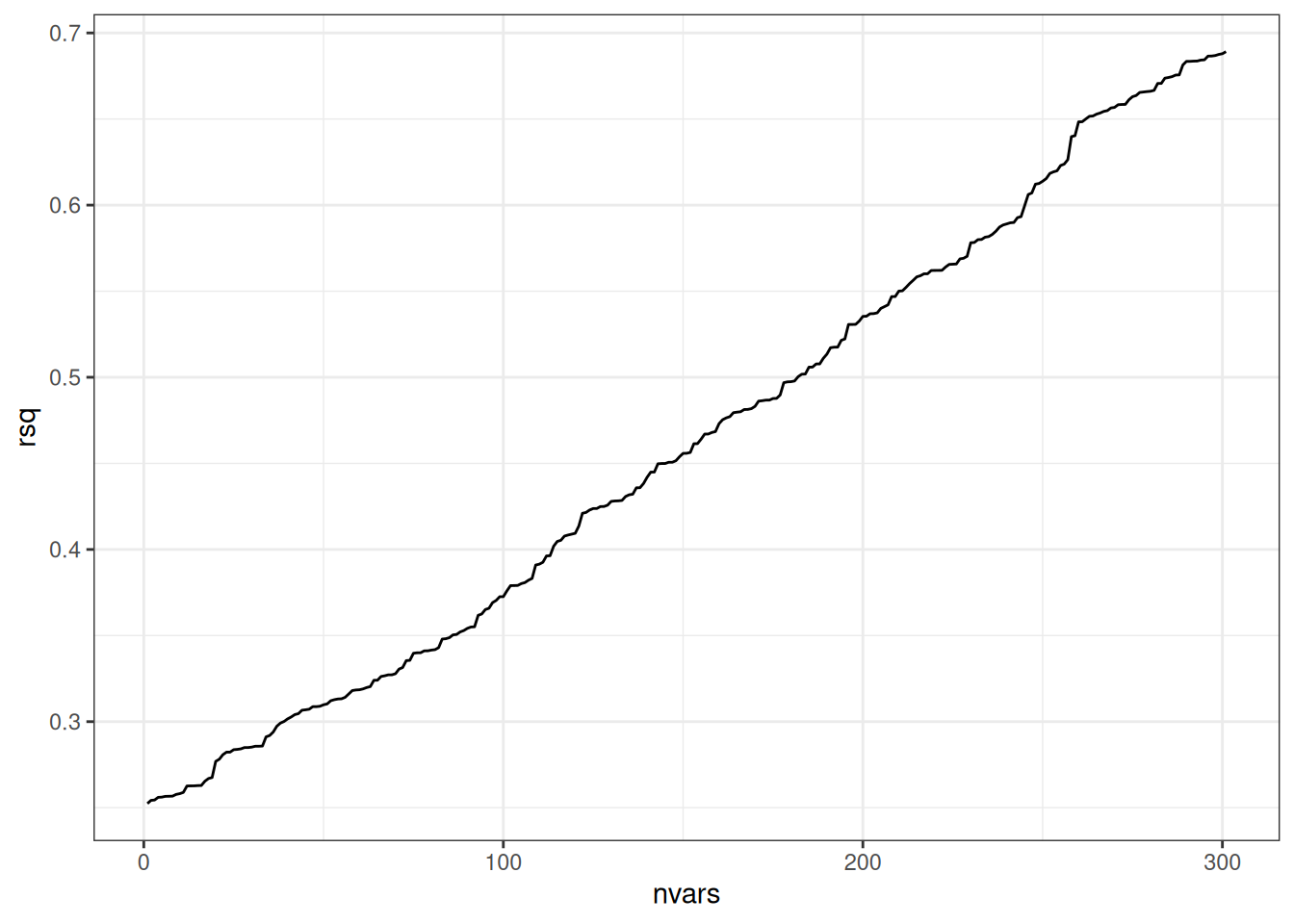
The beginning of the line on the left represents the R-squared value when using the one predictor variable that actually has any true relation with the response variable.
When we add on additional predictors (useless ones), R-squared always increases.
4.24.3 Adjusted \(R^2\) (More conservative)
\[R^2_{adj} = 1 - (1-R^2)\frac{n-1}{n-p-1}\] This is supposed to correct for the fact that \(R^2\) always increases with a greater number of variables (penalizes for the complexity of the model).
Here’s a table for most of the models we’ve discussed so far. It has both the adjusted and unadjusted form.
     model       Rsq    AdjRsq
1   fullLm 0.5030783 0.3767423
2 redModel 0.4176079 0.3519246
3     cor1 0.2671452 0.2621598
4     cor2 0.3275478 0.3183361
5     cor3 0.3476621 0.3341654
6     cor4 0.3508866 0.3328556
7     cor5 0.3514271 0.3287497
8     cor6 0.3943409 0.3687496
But… it doesn’t necessarily. Don’t trust it either.
4.24.4 Predicted \(R^2\) (Even more conservative)
Predicted R-squared or as I will write \(R^2{pred}\) is another play on the same idea as \(R^2\), except for it is based on taking out an observation, computing the regression model without it, then seeing how well the model predicts the left out value.
You can get it via the olsrr package using the ols_pred_rsq() function. The input is your model.
For instance, let us compare this to \(R^2\) from the performance package.
r2(fullLm)# R2 for Linear Regression
R2: 0.503
adj. R2: 0.377library(olsrr)
ols_pred_rsq(fullLm)[1] 0.1258262That’s a lot worse than the 0.503 for the unadjusted R-Squared
Here’s a new table including predicted R-squared
     model       Rsq    AdjRsq   PredRsq
1   fullLm 0.5030783 0.3767423 0.1258262
2 redModel 0.4176079 0.3519246 0.2264297
3     cor1 0.2671452 0.2621598 0.2445699
4     cor2 0.3275478 0.3183361 0.2929179
5     cor3 0.3476621 0.3341654 0.3003604
6     cor4 0.3508866 0.3328556 0.2948558
7     cor5 0.3514271 0.3287497 0.2818233
8 cor6 0.3943409 0.3687496 0.3218613- \(R^2\) only tells how well the model works on the data you have (overfitting kills its utility).
- \(R^2_{adj}\) tries to make an attempt at saying how well the model would work on the wider population/future observations.
- \(R^2_{pred}\) is probably the best measure of how well your model will actually work with new data.
- NONE of these are perfect so use these tools with caution and care.
4.24.5 Akaike Information Criterion AIC
One last point of discussion will be the Akaike Information Criterion.
\[AIC = 2(p+1) + n\log(SSE/n) - C\]
There’s a lot of theory behind this one and the Bayesian Information Criterion (BIC)
\[BIC = (p+1)\ln(n) + n\log(SSE/n) - C\]
This is where things get more confusing since AIC and BIC are numbers where SMALLER IS BETTER.
We will just be looking at AIC
     model       Rsq    AdjRsq   PredRsq      AIC
1   fullLm 0.5030783 0.3767423 0.1258262 183.0882
2 redModel 0.4176079 0.3519246 0.2264297 176.7362
3     cor1 0.2671452 0.2621598 0.2445699 182.9770
4     cor2 0.3275478 0.3183361 0.2929179 172.1605
5     cor3 0.3476621 0.3341654 0.3003604 169.6356
6     cor4 0.3508866 0.3328556 0.2948558 170.8973
7     cor5 0.3514271 0.3287497 0.2818233 172.7732
8     cor6 0.3943409 0.3687496 0.3218613 164.5730
Different measures will tell you different things.
Here \(R^2_{pred}\) and AIC agree that the cor6 model is the best.
cor6 <- lm(suicide_rate ~ self_harm_persons + opiates + marital_breakup +
             children_leaving_care + depression + homeless, phe)
So is that the one we use?
It’s not that simple.
4.25 Variable Selection Methods: Problems and Pitfalls
- Variable selection = methods for choosing which predictor variables to include in statistical models
- Focus on stepwise regression as a common but problematic approach
- Stepwise selection: automated process of adding/removing variables based on statistical significance (p-values and model fit)
4.25.1 Major Problems with Stepwise Selection
4.25.1.1 1. Biased R-squared Values
- R-squared values are inflated
- Makes model appear to explain more variation than it actually does
- Gives false confidence in model’s predictive ability
4.25.1.2 2. Invalid Statistical Inference
- P-values are too small (not valid)
- Confidence intervals are too narrow
- Doesn’t account for multiple testing problem
- Standard errors are biased low
4.25.1.3 3. Biased Regression Coefficients
- Coefficients are biased away from zero
- More likely to select variables with overestimated effects
- Selection process favors chance findings
- True effects may be much smaller than estimated
4.25.1.4 4. Model Instability
- Results highly dependent on sample
- Small changes in data can lead to different variables being selected
- Poor reproducibility
- Different samples likely to produce different models
4.25.2 Example: House Price Prediction
- Scenario: 20 potential predictors of house prices
- First sample might select:
- Square footage
- Number of bathrooms
- Lot size
- Second sample might select completely different variables:
- Age of house
- Number of bedrooms
- Distance to downtown
- Demonstrates instability of selection process
4.25.3 Better Alternatives
4.25.3.1 1. Theory-Driven Selection
- Use subject matter knowledge
- Select variables based on theoretical importance
- Include known important predictors regardless of significance
4.25.3.2 2. Include More Variables
- Keep theoretically important variables
- Don’t eliminate based solely on statistical significance
- Better to include too many than too few important variables
- Degrees of freedom permitting of course!
4.25.3.3 3. Alternative Dimension Reduction Methods
- Principal Components Analysis
- Regularization methods (LASSO, Ridge regression)
- Data reduction techniques that don’t use outcome variable
4.25.4 Key Takeaways
- Avoid automated variable selection methods
- Don’t let computational convenience override good statistical practice
- Complex but theoretically sound models preferred over overly simplified ones
- Statistical significance shouldn’t be the sole criterion for variable inclusion
5 Prespecification of Predictor Complexity in Statistical Modeling
5.1 I. Introduction to Linear Relationships
- Truly linear relationships are rare in real-world data
- Notable exception: Same measurements at different timepoints
- Example: Blood pressure before and after treatment
- Most relationships between predictors and outcomes are nonlinear
- Linear modeling often chosen due to data limitations, not reality
5.2 Problems with Post-Hoc Simplification
5.2.1 Common but Problematic Approaches:
- Examining scatter plots
- Checking descriptive statistics
- Using informal assessments
- Modifying model based on these observations
5.2.2 Key Issue:
- Creates “phantom degrees of freedom”
- Informal assessments use degrees of freedom not accounted for in:
- Standard errors
- P-values
- R² values
5.3 The Prespecification Approach
5.3.1 Core Principles:
- Decide on predictor complexity before examining relationships
- Base decisions on:
- Effective sample size
- Prior knowledge
- Expected predictor importance
- Maintain decisions regardless of analysis results
5.3.2 Benefits:
- More reliable statistical inference
- Better representation of uncertainty
- Prevention of bias from data-driven simplification
5.4 Practical Implementation
5.4.1 Guidelines for Complexity:
- Allow more complex representations for:
- Stronger expected relationships
- Larger effective sample sizes
- More important predictors
5.4.2 Examples of Implementation:
- Using splines with more knots for important predictors
- Scaling complexity to sample size
- Matching complexity to theoretical importance
5.5 Validation and Testing
5.5.1 Allowed Practices:
- Graphing estimated relationships
- Performing nonlinearity tests
- Presenting results to readers
5.5.2 Important Rule:
- Maintain prespecified complexity even if simpler relationships appear adequate
5.6 The Directional Principle
5.6.1 Key Concepts:
- Moving simple → complex
- Degrees of freedom properly increase
- Statistical tests maintain distribution
- Moving complex → simple
- Requires special adjustments
- May compromise statistical validity
5.7 Importance and Impact
5.7.1 Benefits of Prespecification:
- Prevents optimistic performance estimates
- Maintains valid statistical inference
- Provides reliable predictions
- Avoids data-driven simplification bias
5.7.2 Trade-offs:
- May appear conservative
- Slight overfitting preferred to spurious precision
5.8 Summary
- Prespecify predictor complexity based on prior knowledge
- Avoid data-driven simplification
- Maintain statistical validity through consistent approach
- Better to slightly overfit than create spuriously precise estimates
5.9 Sample Size Requirements & Overfitting in Regression Models
5.9.1 Definition
- Overfitting occurs when model complexity exceeds data information content
- Results in:
- Inflated measures of model performance (e.g., R²)
- Poor prediction on new data
- Model fits noise rather than signal
5.9.1.1 Visual Example
Consider two models of the same data:
Simple model:    y ~ x
Overfit model:   y ~ x + x² + x³ + x⁴ + ...
5.9.2 The m/15 Rule
5.9.2.1 Limiting Sample Size (m)
| Type of Response | Limiting Sample Size (m) |
|---|---|
| Continuous | Total sample size (n) |
| Binary | min(n₁, n₂) smaller group |
| Ordinal (k categories) | n - (1/n)Σnᵢ³ |
| Survival time | Number of events/failures |
5.9.2.2 Basic Rule
- Number of parameters (p) should be < m/15
- Some situations require more conservative p < m/20
- Less conservative p < m/10 possible
5.9.3 Counting Parameters
5.9.3.1 Include ALL of these in your count:
- Main predictor variables
- Nonlinear terms
- Interaction terms
- Dummy variables for categorical predictors (k-1)
5.9.3.2 Example Parameter Count
Model components:
- Age (nonlinear, 3 knots) = 2 parameters
- Sex (binary) = 1 parameter
- Treatment (3 categories) = 2 parameters
- Age × Treatment interaction = 4 parameters
Total = 9 parameters
5.9.4 Special Considerations
5.9.4.1 Need More Conservative Ratios When:
- Predictors have narrow distributions
- e.g., age range 30-45 years only
- Highly unbalanced categorical variables
- e.g., 95% in one category
- Clustered measurements
- Small effect sizes expected
5.9.5 Practical Example
5.9.5.1 Binary Outcome Study
Study population:
- 1000 total patients
- 100 heart attacks
- 900 no heart attacks

Calculations:
m = min(100, 900) = 100
Maximum parameters = 100/15 ≈ 6-7
5.9.6 Alternative Approaches
5.9.6.1 Other Methods to Assess/Prevent Overfitting:
- Shrinkage estimates
- Cross-validation
- Bootstrap validation
- Penalized regression methods
5.9.7 Sample Size for Variance Estimation
- Need ~70 observations for ±20% precision in \(\sigma\) estimate
- Affects all standard errors and p-values
- Critical for reliable inference
5.9.8 Key Takeaways
- Count Everything: Include all terms in parameter count
- Be Conservative: Use m/15 as starting point
- Consider Context: Adjust for data peculiarities
- Validate: Use shrinkage or cross-validation
- Simplify: Prefer simpler models when in doubt
5.9.9 Practice Problems
Calculate maximum parameters for:
- 500 patients, continuous outcome
- 1000 patients, 150 events (survival)
- 300 patients, 50/250 binary outcome
Count parameters in model:
y ~ age + age² + sex + treatment*race
where treatment has 3 levels and race has 4 levels
5.10 Shrinkage in Statistical Models: Understanding the Basics
5.10.1 Introduction
- Statistical models can suffer from overfitting
- Overfitting: model performs well on training data but poorly on new data
- Similar to memorizing test answers without understanding concepts
- Need methods to make models more reliable and generalizable
5.10.2 What is Shrinkage?
- Technique to prevent overfitting
- Makes model predictions more conservative and reliable
- Acts like a “leash” on model coefficients
- Helps handle regression to the mean
5.10.3 Example
- Study of 10 different medical treatments
- Some treatments appear very effective by chance
- When tested on new patients, effects usually less extreme
- Natural tendency for extreme results to move toward average
- This movement toward average is “shrinkage”
5.10.4 Key Shrinkage Methods
5.10.4.1 1. Ridge Regression
- Adds penalty to prevent large coefficients
- Characteristics:
- Like rubber band pulling coefficients toward zero
- Keeps all variables in model
- Reduces size of effects
- Ideal for correlated predictors
5.10.4.2 2. LASSO Regression
- Least Absolute Shrinkage and Selection Operator
- Characteristics:
- Can force coefficients to exactly zero
- Performs variable selection
- Creates simpler models
- Good for identifying important variables
5.10.5 Benefits of Shrinkage
- More stable predictions
- Better performance on new data
- Protection against overfitting
- More reliable assessment of variable importance
5.10.6 Key Takeaway
- Shrinkage represents statistical humility
- Prevents extreme predictions based on limited data
- Makes models more reliable and practical
5.11 Data Reduction Methods
5.11.1 Definition
- Process of reducing number of parameters in statistical models
- Focus on dimension reduction without using response variable Y
- “Unsupervised” approach to prevent overfitting
5.11.2 Purpose
- Improve model stability
- Reduce overfitting
- Maintain statistical inference validity
- Handle situations with many predictors relative to sample size
5.11.3 Redundancy Analysis
- Core Concept
- Identifies predictors well-predicted by other predictors
- Removes redundant variables systematically
- Implementation Process
- Convert predictors to appropriate forms
- Continuous → restricted cubic splines
- Categorical → dummy variables
- Use OLS for prediction
- Remove highest R² predictors
- Iterate until threshold reached
- Convert predictors to appropriate forms
5.11.4 Variable Clustering
- Purpose
- Group related predictors
- Identify independent dimensions
- Simplify model structure
- Methods
- Statistical clustering with correlations
- Principal component analysis (oblique rotation)
- Hierarchical cluster analysis
- Important Considerations
- Use robust measures for skewed variables
- Consider rank-based measures
- Hoeffding’s D for non-monotonic relationships
5.11.5 Variable Transformation and Scaling
- Key Methods
- Maximum Total Variance (MTV)
- Maximum Generalized Variance (MGV)
- Process Goals
- Optimize variable transformations
- Maximize relationships between predictors
- Reduce complexity
- Benefits
- Fewer nonlinear terms needed
- Better interpretability
- More meaningful combinations
5.11.6 Simple Scoring of Variable Clusters
- Approaches
- First principal component
- Weighted sums
- Expert-assigned severity points
- Common Applications
- Binary predictor groups
- Hierarchical scoring systems
- Implementation-focused solutions
5.12 Implementation Guidelines
5.12.1 Best Practices
- Prioritize subject matter knowledge
- Validate without response variable
- Use independent data for validation
- Document reduction decisions
- Balance simplicity vs. information
5.12.2 Recommended Workflow
- Start with redundancy analysis
- Apply variable clustering
- Transform within clusters if needed
- Create simple scores where appropriate
- Validate each step
5.13 Key Considerations
5.13.1 Advantages
- Prevents overfitting
- Maintains statistical validity
- Improves model stability
- Enhances interpretability
5.13.2 Limitations
- Potential information loss
- Trade-off with complexity
- Need for validation
5.14 Discussion Points
5.14.1 Critical Questions
- Choosing between methods
- Determining optimal clusters
- Balancing complexity and interpretability
5.14.2 Implementation Challenges
- Deciding on thresholds
- Handling mixed variable types
- Validating reduction decisions
5.14.3 Remarks
- Essential for stable modeling with many predictors
- Requires thoughtful method combination
- Focus on maintaining predictive power
- Ensure statistical validity
5.15 Data Reduction Techniques Examples
First, let’s load the required packages and prepare our data:
library(Hmisc)
library(rms)
library(pcaPP)

# Read the data
df <- read.csv(here::here(
  "datasets",
"phe.csv"))- We have 149 rows of data
- We want to investigate the continuous outcome of
suicide_rate - m/15 rule: we can only have about 10 parameters in the model (we could be more liberal in loosen it to 15 variables)
5.15.1 1. Redundancy Analysis
Redundancy analysis helps identify predictors that can be well-predicted from other variables:
# Perform redundancy analysis
df2 = df %>% dplyr::select(-suicide_rate)
redun_result <- redun(~ .,
                      data=df, r2=0.6)

# Print results
redun_result
Redundancy Analysis

~.

n: 149  p: 31   nk: 3

Number of NAs:   0

Transformation of target variables forced to be linear

R-squared cutoff: 0.6   Type: ordinary

R^2 with which each variable can be predicted from all other variables:

        children_youth_justice       adult_carers_isolated_18
                         0.474                          0.634
adult_carers_isolated_all_ages      adult_carers_not_isolated
                         0.612                          0.769
                 alcohol_rx_18            alcohol_rx_all_ages
                         0.965                          0.998
          alcohol_admissions_f            alchol_admissions_m
                         0.999                          1.000
          alcohol_admissions_p          children_leaving_care
                         0.686                          0.832
                    depression                 domestic_abuse
                         0.738                          0.729
              self_harm_female                 self_harm_male
                         1.000                          1.000
             self_harm_persons                        opiates
                         1.000                          0.952
            lt_health_problems                lt_unepmloyment
                         0.945                          0.876
         looked_after_children                marital_breakup
                         0.889                          0.706
               old_pople_alone                          alone
                         0.956                          0.906
      self_reported_well_being                            smi
                         0.520                          0.859
                social_care_mh                       homeless
                         0.513                          0.790
                    alcohol_rx             drug_rx_non_opiate
                         0.761                          0.787
                drug_rx_opiate                   suicide_rate
                         0.658                          0.639
                  unemployment
                         0.926

Rendundant variables:

self_harm_persons alchol_admissions_m alcohol_rx_all_ages alcohol_rx_18
old_pople_alone self_harm_male unemployment looked_after_children
lt_health_problems smi drug_rx_non_opiate opiates children_leaving_care
alcohol_admissions_f homeless self_harm_female


Predicted from variables:

children_youth_justice adult_carers_isolated_18
adult_carers_isolated_all_ages adult_carers_not_isolated
alcohol_admissions_p depression domestic_abuse lt_unepmloyment
marital_breakup alone self_reported_well_being social_care_mh
alcohol_rx drug_rx_opiate suicide_rate

        Variable Deleted   R^2
1      self_harm_persons 1.000
2    alchol_admissions_m 1.000
3    alcohol_rx_all_ages 0.978
4          alcohol_rx_18 0.960
5        old_pople_alone 0.950
6         self_harm_male 0.927
7           unemployment 0.896
8  looked_after_children 0.866
9     lt_health_problems 0.802
10                   smi 0.783
11    drug_rx_non_opiate 0.727
12               opiates 0.718
13 children_leaving_care 0.704
14  alcohol_admissions_f 0.684
15              homeless 0.663
16      self_harm_female 0.600
                                                            R^2 after later deletions
1           1 1 1 1 0.987 0.987 0.986 0.986 0.986 0.985 0.985 0.984 0.981 0.981 0.625
2   0.997 0.997 0.997 0.996 0.996 0.996 0.996 0.996 0.996 0.996 0.996 0.7 0.696 0.665
3       0.978 0.978 0.977 0.977 0.976 0.974 0.973 0.972 0.972 0.972 0.717 0.713 0.677
4             0.959 0.955 0.952 0.951 0.951 0.947 0.947 0.792 0.787 0.755 0.751 0.742
5                    0.949 0.941 0.941 0.83 0.809 0.801 0.765 0.765 0.753 0.731 0.722
6                          0.925 0.923 0.921 0.92 0.917 0.915 0.912 0.895 0.891 0.636
7                                0.892 0.888 0.883 0.883 0.878 0.867 0.856 0.85 0.848
8                                      0.862 0.86 0.859 0.853 0.777 0.755 0.751 0.722
9                                           0.794 0.792 0.783 0.782 0.768 0.753 0.733
10                                                0.781 0.746 0.741 0.724 0.713 0.704
11                                                      0.724 0.718 0.717 0.716 0.702
12                                                            0.712 0.691 0.689 0.673
13                                                                  0.689 0.674 0.637
14                                                                        0.681 0.656
15                                                                              0.657
16
As with our section on multicollinarity, we can see that a number of variables are redundant. If we were to remove all these variables we would at least satisfy m/10 which is a bit more liberal than the m/15 guidance.
5.15.2 2. Variable Clustering
Let’s perform hierarchical clustering on our variables to identify related groups:
# Perform variable clustering
vc <- varclus(~ .,
              data=df2, sim= 'hoeffding')

# Plot dendrogram
plot(vc)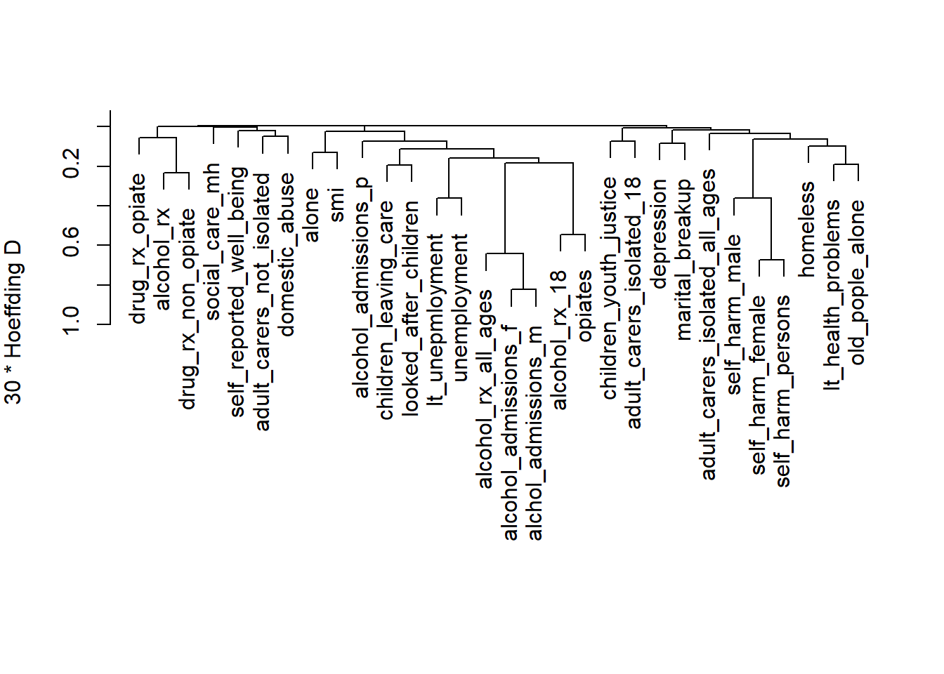
- We can see a lot of the variables clustering together
5.15.3 3. Principal Components Analysis
Let’s examine the data structure using PCA:
# Perform PCA
pca_result <- princomp(df2, cor=TRUE)

# Scree plot
plot(pca_result, type="lines", main="Scree Plot")
abline(h=1, lty=2, col="red")  # Kaiser criterion line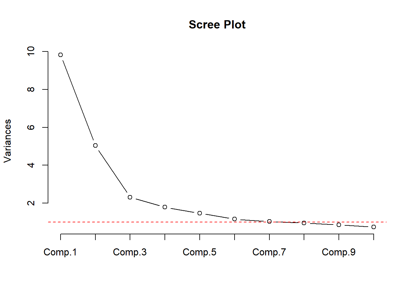
# Print variance explained by first few components
summary(pca_result, loadings=TRUE, cutoff=0.3)
Importance of components:
Comp.1 Comp.2 Comp.3 Comp.4 Comp.5
Standard deviation 3.1327307 2.2436841 1.51857984 1.33713169 1.21224371
Proportion of Variance 0.3271334 0.1678039 0.07686949 0.05959737 0.04898449
Cumulative Proportion 0.3271334 0.4949373 0.57180682 0.63140419 0.68038869
Comp.6 Comp.7 Comp.8 Comp.9 Comp.10
Standard deviation 1.07625280 1.01836888 0.9747646 0.92320127 0.86023787
Proportion of Variance 0.03861067 0.03456917 0.0316722 0.02841002 0.02466697
Cumulative Proportion 0.71899936 0.75356853 0.7852407 0.81365075 0.83831772
Comp.11 Comp.12 Comp.13 Comp.14 Comp.15
Standard deviation 0.76164102 0.74326524 0.70575177 0.67895928 0.65072428
Proportion of Variance 0.01933657 0.01841477 0.01660285 0.01536619 0.01411474
Cumulative Proportion 0.85765429 0.87606907 0.89267192 0.90803811 0.92215284
Comp.16 Comp.17 Comp.18 Comp.19 Comp.20
Standard deviation 0.62502778 0.57314172 0.56636534 0.55357002 0.478567350
Proportion of Variance 0.01302199 0.01094971 0.01069232 0.01021466 0.007634224
Cumulative Proportion 0.93517484 0.94612455 0.95681687 0.96703153 0.974665755
Comp.21 Comp.22 Comp.23 Comp.24
Standard deviation 0.473155304 0.413788556 0.340046283 0.302671397
Proportion of Variance 0.007462531 0.005707366 0.003854382 0.003053666
Cumulative Proportion 0.982128287 0.987835652 0.991690035 0.994743701
Comp.25 Comp.26 Comp.27 Comp.28
Standard deviation 0.250796490 0.224198463 0.174227171 0.1176538993
Proportion of Variance 0.002096629 0.001675498 0.001011837 0.0004614147
Cumulative Proportion 0.996840330 0.998515828 0.999527665 0.9999890799
Comp.29 Comp.30
Standard deviation 1.669952e-02 6.980650e-03
Proportion of Variance 9.295803e-06 1.624316e-06
Cumulative Proportion 9.999984e-01 1.000000e+00
Loadings:
Comp.1 Comp.2 Comp.3 Comp.4 Comp.5 Comp.6 Comp.7
children_youth_justice 0.378 0.580
adult_carers_isolated_18 0.413 0.307
adult_carers_isolated_all_ages
adult_carers_not_isolated
alcohol_rx_18
alcohol_rx_all_ages
alcohol_admissions_f
alchol_admissions_m
alcohol_admissions_p
children_leaving_care
depression
domestic_abuse 0.342
self_harm_female
self_harm_male
self_harm_persons
opiates
lt_health_problems
lt_unepmloyment
looked_after_children
marital_breakup
old_pople_alone 0.338
alone -0.434
self_reported_well_being 0.381
smi -0.366
social_care_mh 0.488
homeless -0.325
alcohol_rx -0.543
drug_rx_non_opiate -0.558
drug_rx_opiate -0.397
unemployment
Comp.8 Comp.9 Comp.10 Comp.11 Comp.12 Comp.13
children_youth_justice
adult_carers_isolated_18
adult_carers_isolated_all_ages 0.351 -0.499 -0.301
adult_carers_not_isolated
alcohol_rx_18
alcohol_rx_all_ages
alcohol_admissions_f
alchol_admissions_m
alcohol_admissions_p -0.378
children_leaving_care
depression 0.340 0.373
domestic_abuse -0.397 0.304
self_harm_female
self_harm_male
self_harm_persons
opiates 0.335
lt_health_problems
lt_unepmloyment
looked_after_children
marital_breakup -0.316 -0.366 0.442
old_pople_alone -0.344
alone
self_reported_well_being 0.605 -0.374
smi
social_care_mh -0.618
homeless
alcohol_rx
drug_rx_non_opiate
drug_rx_opiate 0.312 -0.320
unemployment
Comp.14 Comp.15 Comp.16 Comp.17 Comp.18 Comp.19
children_youth_justice 0.376
adult_carers_isolated_18 -0.505 -0.378
adult_carers_isolated_all_ages 0.304
adult_carers_not_isolated -0.390 0.510 -0.459
alcohol_rx_18
alcohol_rx_all_ages
alcohol_admissions_f
alchol_admissions_m
alcohol_admissions_p 0.376 -0.366
children_leaving_care 0.393
depression -0.304 0.406 -0.387
domestic_abuse 0.311
self_harm_female
self_harm_male
self_harm_persons
opiates -0.305
lt_health_problems
lt_unepmloyment -0.448 -0.334
looked_after_children
marital_breakup
old_pople_alone
alone
self_reported_well_being
smi
social_care_mh
homeless 0.483
alcohol_rx
drug_rx_non_opiate 0.338
drug_rx_opiate -0.382
unemployment
Comp.20 Comp.21 Comp.22 Comp.23 Comp.24 Comp.25
children_youth_justice
adult_carers_isolated_18
adult_carers_isolated_all_ages
adult_carers_not_isolated
alcohol_rx_18
alcohol_rx_all_ages
alcohol_admissions_f
alchol_admissions_m
alcohol_admissions_p
children_leaving_care -0.469
depression
domestic_abuse
self_harm_female 0.495
self_harm_male -0.668
self_harm_persons
opiates
lt_health_problems 0.423
lt_unepmloyment 0.422
looked_after_children 0.634 0.429
marital_breakup -0.370
old_pople_alone 0.307
alone -0.441
self_reported_well_being
smi 0.561 -0.314
social_care_mh
homeless 0.349
alcohol_rx 0.525
drug_rx_non_opiate -0.316 -0.454
drug_rx_opiate
unemployment -0.659
Comp.26 Comp.27 Comp.28 Comp.29 Comp.30
children_youth_justice
adult_carers_isolated_18
adult_carers_isolated_all_ages
adult_carers_not_isolated
alcohol_rx_18 0.342 -0.625
alcohol_rx_all_ages -0.760
alcohol_admissions_f 0.590 0.513
alchol_admissions_m -0.806
alcohol_admissions_p
children_leaving_care
depression
domestic_abuse
self_harm_female 0.487
self_harm_male -0.353 0.338
self_harm_persons -0.804
opiates -0.379 0.435
lt_health_problems 0.479
lt_unepmloyment
looked_after_children
marital_breakup
old_pople_alone -0.488
alone
self_reported_well_being
smi
social_care_mh
homeless
alcohol_rx
drug_rx_non_opiate
drug_rx_opiate
unemployment -0.312 5.15.4 4. Sparse Principal Components Analysis
Using pcaPP for robust sparse PCA.
# Perform sparse PCA
sparse_pca <- sPCAgrid(df2, k=10, method = 'sd' ,
center =mean , scale =sd , scores =TRUE ,
maxiter =10)

# Plot variance explained
plot(sparse_pca,type = 'lines' , main= ' ')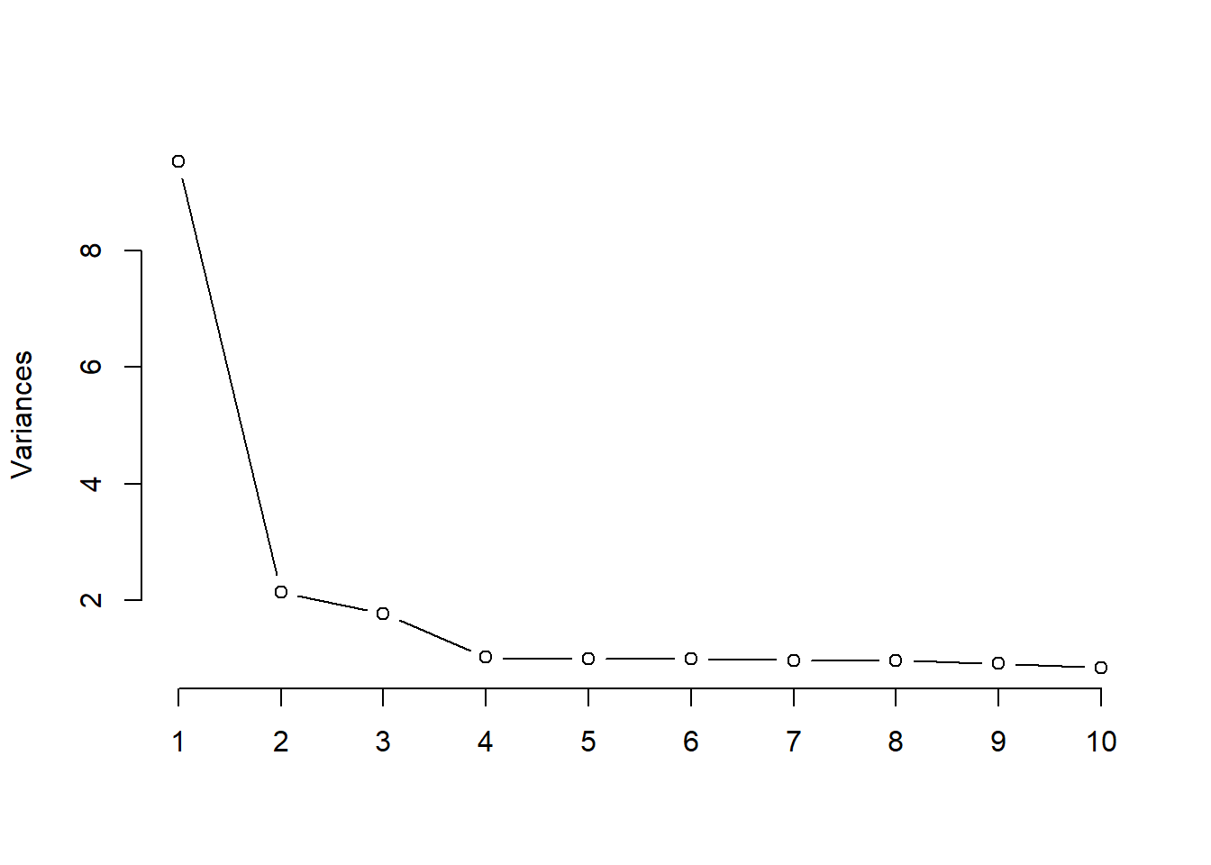
# Print loadings
print(sparse_pca$loadings)
Loadings:
                               Comp.1 Comp.2 Comp.3 Comp.4 Comp.5 Comp.6 Comp.7
children_youth_justice                                             1.000
adult_carers_isolated_18
adult_carers_isolated_all_ages         0.464
adult_carers_not_isolated       0.252
alcohol_rx_18                   0.295
alcohol_rx_all_ages             0.305
alcohol_admissions_f            0.295
alchol_admissions_m             0.303
alcohol_admissions_p            0.161
children_leaving_care           0.248
depression                      0.111
domestic_abuse                  0.106                                     0.791
self_harm_female                0.131               -0.264
self_harm_male                  0.222
self_harm_persons               0.176
opiates                         0.278
lt_health_problems              0.210
lt_unepmloyment                 0.226
looked_after_children           0.300
marital_breakup                 0.113
old_pople_alone                        0.636
alone                           0.122                                    -0.607
self_reported_well_being                             0.965
smi                             0.122
social_care_mh                                              1.000
homeless                              -0.613
alcohol_rx                                    0.707
drug_rx_non_opiate                            0.707
drug_rx_opiate
unemployment                    0.234
                               Comp.8 Comp.9 Comp.10
children_youth_justice
adult_carers_isolated_18
adult_carers_isolated_all_ages
adult_carers_not_isolated
alcohol_rx_18
alcohol_rx_all_ages
alcohol_admissions_f
alchol_admissions_m
alcohol_admissions_p                         -0.574
children_leaving_care
depression                      0.903
domestic_abuse
self_harm_female
self_harm_male
self_harm_persons                      0.444
opiates
lt_health_problems
lt_unepmloyment
looked_after_children
marital_breakup                               0.819
old_pople_alone
alone
self_reported_well_being
smi
social_care_mh
homeless
alcohol_rx
drug_rx_non_opiate
drug_rx_opiate                         0.896
unemployment                   -0.426

               Comp.1 Comp.2 Comp.3 Comp.4 Comp.5 Comp.6 Comp.7 Comp.8 Comp.9
SS loadings     1.000  1.000  1.000  1.000  1.000  1.000  1.000  1.000  1.000
Proportion Var  0.033  0.033  0.033  0.033  0.033  0.033  0.033  0.033  0.033
Cumulative Var  0.033  0.067  0.100  0.133  0.167  0.200  0.233  0.267  0.300
               Comp.10
SS loadings      1.000
Proportion Var   0.033
Cumulative Var   0.333
Like are variable clutstering, we can see that lots of variables load onto the first principal component. We could add component 1 to our regression model and keep the rest of the variables (not those loaded on comp. 1).
However, let’s instead use stepwise regression only on the preditors in combination with sparse PCA to select variables for 10 components in our model.
- Stepwise here tells us which predictors that load onto each PC are needed to predict that pc
spca1 <- princmp(df2, sw = TRUE ,
                 k = 10,
                 kapprox = 10,
                 method = "sparse",
                 cor = TRUE,
                 nvmax = 30)

print(spca1)
Sparse Principal Components Analysis
Stepwise Approximations to PCs With Cumulative R^2
PC 1
alchol_admissions_m (0.975) + self_harm_persons (0.999) +
looked_after_children (1)
PC 2
adult_carers_isolated_all_ages (0.759) + homeless (0.978) +
old_pople_alone (1)
PC 3
drug_rx_non_opiate (0.89) + alcohol_rx (1)
PC 4
self_harm_female (1)
PC 5
adult_carers_isolated_18 (0.861) + self_harm_female (1)
PC 6
self_harm_female (0.993) + self_reported_well_being (1)
PC 7
social_care_mh (1)
PC 8
children_youth_justice (1)
PC 9
domestic_abuse (0.872) + alone (1)
PC 10
depression (0.875) + unemployment (0.999) + old_pople_alone (1)We get 10 components, some with many predictors, some with only one.
5.15.5 Put it all together
Using theory, we could decide to create cluster scores for some of these components, while others with only 2 variables we might want to just eliminate one of the variables.
For those that we want to have a composite score, we can use the first principal component of their scores. Or, if we want to use this scoring outside of this context we can get a regression model on the first PC.
Let me demonstrate with our first component from the sparse PCA.
# Get pc scores for the first sparse PC variables
pc1_scores = princmp(df2[,c(names(spca1$sw[[1]]))],
                     method = "regular",
                     cor = TRUE)$scores[,1]
df2$pc1_scores = pc1_scores

mod1 = lm(pc1_scores~alchol_admissions_m + self_harm_persons , data = df2)

parameters::parameters(mod1) |> print_md()| Parameter | Coefficient | SE | 95% CI | t(146) | p |
|---|---|---|---|---|---|
| (Intercept) | -6.53 | 0.18 | (-6.88, -6.17) | -36.38 | < .001 |
| alchol admissions m | 3.63e-03 | 1.47e-04 | (3.34e-03, 3.92e-03) | 24.70 | < .001 |
| self harm persons | 9.09e-03 | 4.38e-04 | (8.22e-03, 9.95e-03) | 20.75 | < .001 |
Now, we could report those regression coefficients to get a pretty reasonable estimate of the scoring for that component of the model.
Now, let’s get the second and third scores as well.
# Get pc scores for the second sparse PC variables
pc2_scores = princmp(df2[,c(names(spca1$sw[[2]]))],
                     method = "regular",
                     cor = TRUE)$scores[,1]

df2$pc2_scores = pc2_scores

pc3_scores = princmp(df2[,c(names(spca1$sw[[3]]))],
                     method = "regular",
                     cor = TRUE)$scores[,1]

df2$pc3_scores = pc3_scores
For the rest, we will simplify things a bit and just use the first variable of the remaining 10 sparse PCA components.
Let’s now fit a model based using our 3 PCs and the 7 other variables we selected.
df_all = df2 %>%
  select(pc1_scores, pc2_scores, pc3_scores,
         self_harm_female,
         adult_carers_isolated_18,
         self_harm_female,
         social_care_mh,
         children_youth_justice,
         domestic_abuse,
         depression)

df_all$suicide_rate = df$suicide_rate

# 10 predictors, 1 outcome, 149 observations
model_all = lm(
  data = df_all,
  suicide_rate ~ .
)

summary(model_all)
Call:
lm(formula = suicide_rate ~ ., data = df_all)

Residuals:
    Min      1Q  Median      3Q     Max
-4.2067 -1.1131 -0.1051  0.9371  4.1430

Coefficients:
                           Estimate Std. Error t value Pr(>|t|)
(Intercept)               9.6296409  1.6223906   5.935 2.22e-08 ***
pc1_scores                0.5747571  0.1555263   3.696 0.000315 ***
pc2_scores                0.3436984  0.1388871   2.475 0.014539 *
pc3_scores               -0.1009508  0.1084578  -0.931 0.353579
self_harm_female          0.0025597  0.0024544   1.043 0.298819
adult_carers_isolated_18  0.0239721  0.0243409   0.985 0.326408
social_care_mh            0.0010556  0.0004836   2.183 0.030729 *
children_youth_justice   -0.0310969  0.0241586  -1.287 0.200165
domestic_abuse            0.0266173  0.0359734   0.740 0.460599
depression               -0.1202582  0.1114831  -1.079 0.282584
---
Signif. codes:  0 '***' 0.001 '**' 0.01 '*' 0.05 '.' 0.1 ' ' 1

Residual standard error: 1.729 on 139 degrees of freedom
Multiple R-squared:  0.3853,    Adjusted R-squared:  0.3455
F-statistic: 9.681 on 9 and 139 DF,  p-value: 2.122e-11
Now let’s check our assumptions:
check_model(model_all)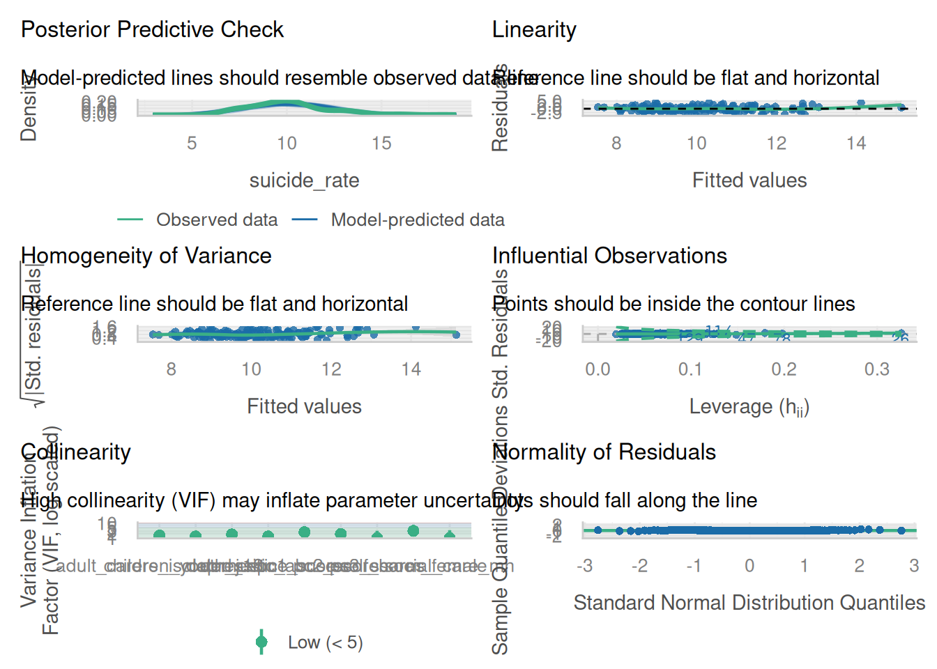
5.15.6 Analysis Summary
From the redundancy analysis, we can identify variables that are highly predictable from others, helping reduce dimensionality while maintaining information.
The variable clustering dendrogram shows natural groupings in our data, which can guide feature selection or creation of composite scores.
The PCA results show how many components are needed to explain a certain percentage of variance in the data.
Sparse PCA provides a more interpretable solution by forcing some loadings to zero while maintaining most of the explained variance.
5.15.7 Recommendations for Data Reduction
Based on these analyses, we can recommend:
Consider combining highly correlated variables within the same cluster into composite scores
Use the first few principal components if dimension reduction is needed while maintaining maximum variance
For interpretability, consider using the sparse PCA solution which provides clearer variable groupings
Remove redundant variables identified in the redundancy analysis on an as needed basis. Justify your choices!
These techniques provide different perspectives on data reduction, and the choice depends on the specific needs of the analysis (interpretability, variance preservation, or prediction accuracy).
5.16 Modern variable selection: ABESS and VSURF
The previous sections built up two related messages. First, naive automated selection (stepwise, “keep the significant ones”) distorts coefficients, breaks the standard errors, and is unstable across samples. Second, shrinkage (ridge and LASSO) is better understood as a variance-reduction tool than as a way to “find the right variables.” This section adds two modern selectors that are genuinely better-behaved than stepwise selection, while being explicit about the line they still cannot cross.
Both methods answer one question, what makes a variable worth keeping?, in very different ways.
- ABESS answers from inside the linear or generalized linear model. It optimizes a penalized fit criterion that counts how many variables are in the model (an \(L_0\) objective), so the “best” subset is the one that fits well without using too many predictors.
- VSURF answers from outside the linear model entirely. It ranks variables by how much they help a random forest predict, then keeps the ones that carry predictive signal.
Note
Read this section against Section 5.16’s predecessors, the Harrell material on the pitfalls of selection and the shrinkage discussion. ABESS and VSURF are more principled than stepwise selection, but neither one escapes the fundamental caveat: once you let the data choose the variables, the usual standard errors and p-values on the model you land on are no longer valid. They are better selectors, not valid inference procedures. That tension is the point, and it supplies most of the “what they cannot do” content below.
5.17 ABESS: adaptive best subset selection
5.17.1 What it is
Best subset selection asks the most direct question possible: of all the ways to pick \(k\) predictors out of \(p\), which subset fits best? Classically this is infeasible because the number of subsets explodes combinatorially. ABESS makes it tractable with a splicing algorithm that iteratively swaps variables into and out of the active set until no swap improves the fit, solving the \(L_0\)-constrained problem in polynomial time (Zhu et al. 2020; Zhu et al. 2022).
Two features make it fit the way this course already thinks about regression:
- It supports linear, logistic, Poisson, Cox, and multi-response models, so it operates directly inside the GLM frame rather than off to the side.
- It tunes the support size (how many variables to keep) automatically with an information criterion (a GIC/EBIC-type penalty), so the analyst does not pick \(k\) by hand.
5.17.2 What it can do
- Return a best-subset solution at a scale where classic exhaustive search is hopeless.
- Avoid the shrinkage bias LASSO imposes on the coefficients it retains. This is the same motivation behind relaxed LASSO, adaptive LASSO, SCAD, and MCP: select with one tool, but do not pay a penalty on the kept coefficients.
- Choose the support size for you, instead of leaving it as a tuning knob.
- Recover the true active set when the design is well-behaved (sparse-eigenvalue or restricted-isometry-type conditions).
5.17.3 What it cannot do
Warning
- Provide valid post-selection inference. If you refit the chosen subset and report the usual standard errors and p-values, you are pretending selection never happened. See Section 5.20.
- Behave well under heavy predictor collinearity. When predictors are redundant, “the best subset” becomes unstable in exactly the way Section 4.21 describes.
- Tell you that many near-equivalent subsets usually exist. ABESS returns one “best” model and hides the selection instability that Harrell has students quantify with bootstrap inclusion frequencies. One clean answer can be more misleading than a messy distribution of answers.
5.18 VSURF: variable selection with random forests
There is no recorded lecture for this topic. The videos below are by Dustin Fife, whose “Quant Psych” channel covers this material well.
5.18.1 What it is
VSURF is a three-step procedure built on random forest permutation importance (Breiman 2001; Genuer et al. 2010, 2015). The importance of a variable is the drop in out-of-bag accuracy when that variable’s values are randomly permuted: if scrambling a variable hurts prediction, the forest was using it.
- Thresholding drops variables whose importance falls below a threshold derived from the noise in the importance estimates.
- Interpretation selects a nested set of variables aimed at understanding the data.
- Prediction refines a smaller set aimed at predictive accuracy.
Note
This is not “machine learning applied to a linear model.” VSURF discards the linear model and fits a forest. Think of it as a model-agnostic, importance-based selection philosophy whose output can inform a downstream linear model, not as a linear-model method itself. A sharp student will notice there is no linear model anywhere inside it, so it is worth saying plainly first.
5.18.2 What it can do
- Capture nonlinearity and interactions in the importance ranking without the analyst specifying them in advance.
- Separate an interpretation set (variables worth understanding) from a smaller prediction set (variables worth keeping for accuracy).
5.18.3 What it cannot do
Warning
- Give effects in interpretable units, or any inference at all. A forest does not hand you a coefficient with a standard error.
- Produce a stable answer. Results depend on
ntreeand on the random seed; rerun it and the selected set can shift. - Avoid importance bias under correlated predictors. Standard permutation importance favors correlated and high-cardinality variables (Strobl et al. 2007); conditional permutation importance is a partial remedy, not a cure.
5.19 Demo: do the methods agree?
The most useful thing to see is that these methods, given the same data, keep different variables. We run LASSO, ABESS, and VSURF on one dataset and line up what each one selects. We use ISLR2::Hitters (predicting a baseball player’s Salary), the canonical best-subset teaching set, because it has a moderate number of predictors with some collinearity.
# setup --------
library(ISLR2)
library(glmnet)
library(abess)
library(VSURF)

set.seed(20260618)

dat <- na.omit(ISLR2::Hitters)
y   <- dat$Salary
x   <- model.matrix(Salary ~ ., data = dat)[, -1]

# lasso (variance-reduction baseline) --------
cv_lasso   <- cv.glmnet(x, y, alpha = 1)
lasso_coef <- coef(cv_lasso, s = "lambda.1se")
lasso_set  <- rownames(lasso_coef)[which(lasso_coef[, 1] != 0)]
lasso_set  <- setdiff(lasso_set, "(Intercept)")

# abess (l0 best subset, support size chosen by IC) --------
fit_abess  <- abess(x, y, family = "gaussian")
abess_best <- extract(fit_abess)
abess_set  <- (abess_best$support.vars)

# vsurf (random forest permutation importance) --------
fit_vsurf    <- VSURF(x = x, y = y,
                      verbose = FALSE)
vsurf_interp <- colnames(x)[fit_vsurf$varselect.interp]
vsurf_pred   <- colnames(x)[fit_vsurf$varselect.pred]

# compare selected sets --------
all_vars <- colnames(x)
comparison <- data.frame(
  variable     = all_vars,
  lasso        = ifelse(all_vars %in% lasso_set,    "Yes", ""),
  abess        = ifelse(all_vars %in% abess_set,    "Yes", ""),
  vsurf_interp = ifelse(all_vars %in% vsurf_interp, "Yes", ""),
  vsurf_pred   = ifelse(all_vars %in% vsurf_pred,   "Yes", "")
)

knitr::kable(comparison, row.names = FALSE)| variable | lasso | abess | vsurf_interp | vsurf_pred |
|---|---|---|---|---|
| AtBat | Yes | |||
| Hits | Yes | Yes | ||
| HmRun | ||||
| Runs | ||||
| RBI | ||||
| Walks | Yes | Yes | ||
| Years | Yes | Yes | ||
| CAtBat | Yes | Yes | ||
| CHits | Yes | Yes | ||
| CHmRun | Yes | |||
| CRuns | Yes | Yes | Yes | |
| CRBI | Yes | Yes | Yes | Yes |
| CWalks | Yes | Yes | ||
| LeagueN | ||||
| DivisionW | Yes | |||
| PutOuts | Yes | Yes | ||
| Assists | ||||
| Errors | ||||
| NewLeagueN |
Reading down Table 5.1, the two linear-model selectors largely agree with each other: LASSO and ABESS both lean on single-season rate stats such as Hits and Walks together with PutOuts and CRBI. VSURF picks an almost disjoint set, dominated by the career cumulative totals (CAtBat, CHits, CHmRun, CRuns, CWalks) plus Years. Across all three methods, essentially the only variable they all keep is CRBI.
The split is not random. The career-total variables are strongly collinear with one another, and random forest permutation importance is biased toward such correlated clusters (the Strobl et al. (2007) effect noted in Section 5.18): the forest spreads its predictive credit across the whole career-stats group, while the \(L_1\) and \(L_0\) linear methods prefer a sparser mix. VSURF’s prediction set is also smaller than its interpretation set by construction, and it shifts if you change ntree or the seed.
Tip
Three reasonable methods, given identical data, keep different variables. That disagreement is the empirical face of selection instability. It is also the reason inference after selection needs care: if the set you would report depends on the method and the seed, then the standard errors computed as if that set were fixed in advance are telling you a story that is too clean to be true.
5.20 A note on inference after selection
Warning
Every method in this section hands you a model and then tempts you to report the usual standard errors and p-values on it. Those numbers are invalid, because selection already consumed information that the inference pretends is still available: the data were used once to choose the variables and a second time to test them, but the test acts as if the variables were fixed in advance. The honest paths are selective-inference methods, which adjust the inference for the fact that selection happened (Berk et al. 2013), and bootstrapping the entire selection procedure, refitting from scratch on each resample, to see how often each variable actually survives. ABESS and VSURF change which variables you select; they do not change this.
5.21 Our model building process
- Look at the full model. Coefficients, residuals, and all.
- Investigate for multicollinearity and find ways to remove variables that may be problematic.
- Look at the full model of the reduced data: coefficients, residuals, and all. You may need to apply a transformation to the \(y\) variable.
- If you think it’s a good fit and can justify using it, you’re done.
- Otherwise you need to start eliminating variables via knowledge of the data or specific experimental questions ideally. If you are purely aiming for a predictive approach, you may try data reduction methods.
- Once you have found a reduced model, examine the residuals for outliers and violation assumptions. Remove outliers only if you can justify it.
- If you don’t have outliers and your assumptions look good, you’re done.
- Check if your variables still remain relevant. You may have to remove or add variables that are now relevant. Use experimental questions or data reduction again…
- Check residuals and outliers again. Hopefully everything looks good.
Every time you messed with something in the model, you need to go back through and check residuals, validity of transformations, etc.
I’ll throw you softballs in this class for the sake of your sanity.