5  Module 5: Generalized Linear Model

Here are some code chunks that setup this chapter

# Need the knitr package to set chunk options
library(knitr)
library(tidyverse)
library(gridExtra)
library(caret)
library(readr)
library(ggfortify)
library(car)
library(performance)
library(see)

It should be noted that depending on the time frame that you may read about “GLMs”, this may refer to two different types of modeling schemes

• GLM \(\to\) General Linear Model: This is the older scheme that now refers to Linear Mixed Models or LMMs. This has more with correlated error terms and “random effects” in model.

• These days GLM refers to Generalized Linear Model. Developed by Nelder, John; Wedderburn, Robert (1972). This takes the concept of a linear model and generalizes it to response variables that do not have a normal distribution. This is what GLM means today. (I haven’t run into an exception, but there might be ones out there depending on the discipline.)

5.1 Components of Linear Model

We will start with the idea of the regression model we have been working.

\[ \mu_{y|x}= \beta_0 + \beta_1 x_1 + \beta_2 x_2 + \dots + \beta_p x_p. \]

• Here we are saying that the mean value of \(y\), \(\mu_{y|x}\), is determined by the values of our predictor variables.

• For making predictions, we have to add in a random component (because no model is perfect).

\[ y = \mu_{y|x} + \epsilon = \beta_0 + \beta_1 x_1 + \beta_2 x_2 + \dots + \beta_p x_p + \epsilon. \]

We have two components here.

1. A deterministic component.

2. A random component: \(\epsilon \sim N(0, \sigma^2)\).

• The random component means that \(Y \sim N(\mu_{y|x}, \sigma^2)\).

• The important part here is that the mean value of \(y\) is assumed to be linearly related to our \(x\) variables.

5.1.1 Introduction to Link Functions

We have tried transformations on data to try to see if we can fix heterogenity and non-linearity issues.

• In Generalized Linear Models these are known as link functions.
• The functions are meant to link a linear model to the distribution of \(y\) or link the distribution of \(y\) to a linear model. (which ever way you want to think about it)
• In the case of linear regression they are supposed to be the link of \(y\) with Normality and linearity.

Example:

\[ \begin{aligned} g(y) &= \log(y) &= \eta_{y|x} + \epsilon = \beta_0 + \beta_1 x_1 + \beta_2 x_2 + \dots + \beta_p x_p + \epsilon \end{aligned} \]

What does this mean for \(y\) itself?

\[ \begin{aligned} Y &= g^{-1}\left( \eta_{y|x} + \epsilon \right) = e^{\eta_{y|x}+ \epsilon}\\ \mu_{y|x} &= e^{\beta_0 + \beta_1 x_1 + \beta_2 x_2 + \dots + \beta_p x_p + \epsilon} \end{aligned} \]

• Another common option is \(g(Y) = Y^p\) where it could be hoped that \(p = 1\) but more often the best \(p\) is not…

5.1.2 Form of Generalized Linear Models

The form of Generalized Linear Models takes the basic form:

• Observations of \(y\) are the result of some probability distribution whose mean (and potentially variance) are determined or correlated with certain “predictor”/x variables.

• The mean value of \(y\) is \(\mu_{y|x}\) and is not linearly related to \(x\), but via the link function it is, i.e., \[g(\mu_{y|x}) = \]

There are now three components we consider:

1. A deterministic component.

2. The probability distribution of \(y\) with some mean \(\mu_{y|x}\) and standard deviation (randomness) \(\sigma_{y|x}\).

• In ordinary linear regression the probability distribution for \(y\) was \[N(\beta_0 + \beta_1 x_1 + \beta_2 x_2 + \dots + \beta_p x_p, \sigma)\]
• Consider \(y\) from a binomial distribution with probability of success \(p(x)\), that is, the probability depends on \(x\). For an individual trial, we have:
  • \(\mu_{y|x} = p(x)\)
  • \(\sigma_{y|x} = \sqrt{p(x)(1-p(x))}\)
  • This makes is so we can no longer just chuck the error term into the linear equation for the mean to represent the randomness.

3. A link function \(g(y)\) such that

\[ \begin{aligned} g\left(\mu_{y|x}\right) &= \eta_{y|x}\\ &= \beta_0 + \beta_1 x_1 + \beta_2 x_2 + \dots + \beta_p x_p \end{aligned} \]

With GLMs, we are now paying attention to a few details.

• \(y\) is not restricted to the normal distributions; that’s the entire point…

• The link function is chosen based on the distribution of \(y\)

  • The distribution of \(y\) determines the form of \(\mu_{y|x}\).

5.1.3 Various Types of GLMs

Distribution of \(Y\)	Support of \(Y\)	Typical Uses	Link Name	Link Function: \(g(y)\)
Normal	\(\left(-\infty, \infty\right)\)	Linear response data	Identity	\(g\left(\mu_{y|x}\right) = \mu_{y|x}\)
Exponentail	\(\left(0, \infty\right)\)	Exponential Processes	Inverse	\(g\left(\mu_{y|x}\right) = \frac{1}{\mu_{y|x}}\)
Poisson	\(0,1,2,\dots\)	Counting	Log	\(g\left(\mu_{y|x}\right) = \log_{y|x}\)
Binomial	\(0,1\)	Classification	Logit	\(g\left(\mu_{y|x}\right) = \text{ln}\left(\frac{\mu_{y|x}}{1-\mu_{y|x}}\right)\)

We will mainly explore Logistic Regression, which uses the Logit function.

This is one of the ways of dealing with Classification.

5.2 Classification Problems, In General.

Classification can be simply define as determing what the outcome is for a discrete random variable.

• An online banking service must be able to determine whether or not a transaction being performed on the site is fraudulent, on the basis of the user’s past tranaction history, balance, an other potential predictors. This a common use of statistical classification known as Fraud detection

• On the basis of DNA sequence data for a number of patients with and without a given disease a biologist would like to figure out which DNA mutations are disease-causing and which are not.

• A person arrives at the emergency room with a set of symptoms that could possiblly be attributed to one of three medical conditions: stroke, drug overdose, epileptic seizure. We would want to choose or classify the person into one of the three categories.

In each of these situations what is the distribution of \(Y =\) the category an indidual falls into?

5.2.1 Odds and log-odds

In classification models, the idea to to estimate the probability of an event occuring for an individual: \(p\).

There are a couple of ways that we assess how likely an event is:

• Odds are \(Odds(p) = \frac{p}{1-p}\)
  • This is the ratio of an event occurring versus it not occurring.
  • This gives a numerical estimate of how many times more likely it is for the event to occur rather than not.
  • \(Odds = 1\) implies a fifty/fifty split: \(p = 0.5\). (Like a coin flip!)
  • \(Odds = d\) where \(d > 1\) implies that the event is \(d\) times more likely to happen than not.
  • For \(d < 0\) the event is \(1/d\) times more likely to NOT happen rather than happen.
• log-odds are taking the logarithm (typically the natural logarithm) of the odds: \(\log(Odds(p)) = log\left(\frac{p}{1-p}\right)\)$
  • In logistic regression, the linear relationship between \(p(x)\) and the predictor variables is assumed to be via \(\log(Odds)\).
  • \(log\left(\frac{p}{1-p}\right) = \beta_0 + \beta_1x_1 + \dots + \beta_kx_k\)

5.3 An Example, Default

We will consider an example where we are interested in predicting whether an individual will default on their credit card payment, on the basis of annual income, monthly credit card balance and student status. (Did I pay my bills… Maybe I should check.)

Default <- read_csv(here::here("datasets","Default.csv"))

# Converting Balance and Income to Thousands of dollars

Default$balance <- Default$balance/1000
Default$income <- Default$income/1000

head(Default)

# A tibble: 6 × 5
   ...1 default student balance income
  <dbl> <chr>   <chr>     <dbl>  <dbl>
1     1 No      No        0.730  44.4 
2     2 No      Yes       0.817  12.1 
3     3 No      No        1.07   31.8 
4     4 No      No        0.529  35.7 
5     5 No      No        0.786  38.5 
6     6 No      Yes       0.920   7.49

• student whether the person is a student or not.
• default is whether they defaulted
• balance is there total balance on their credit cards.
• income is the income of the individual.

5.3.1 A little bit of EDA

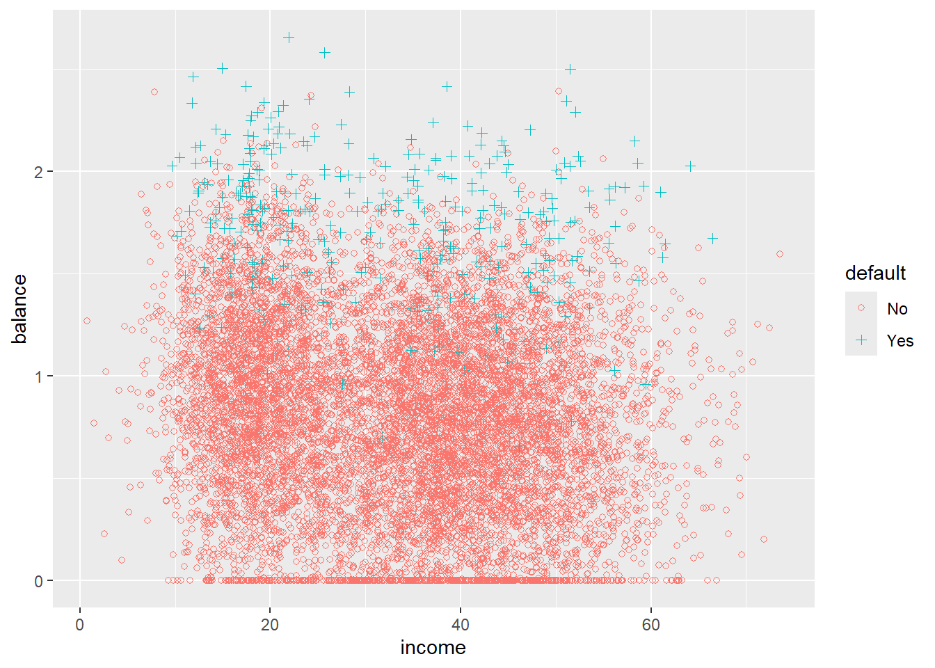
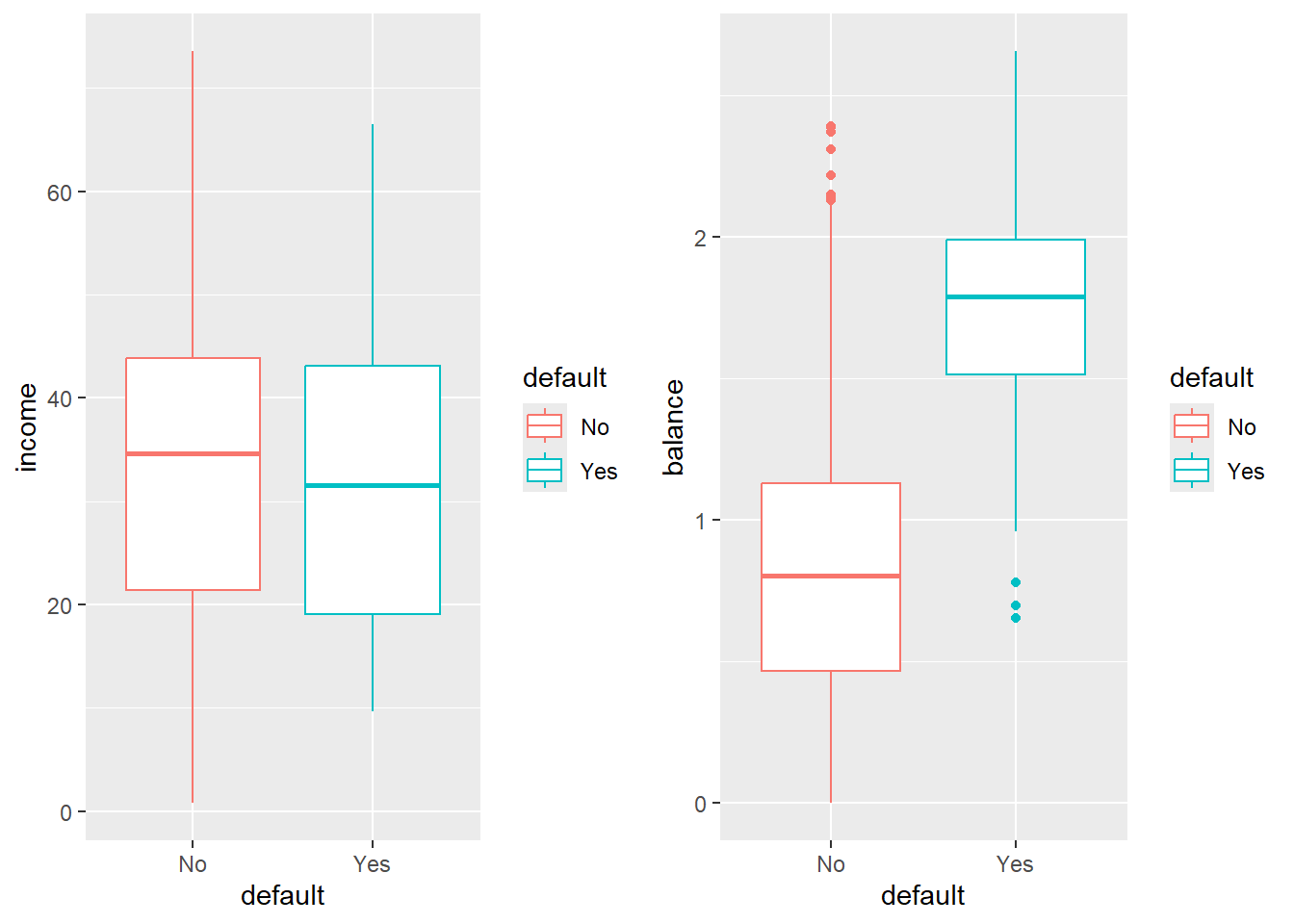
Try to describe what you see.

5.3.2 Logistic Regression

For each individual \(y_i\) we are trying to model if that individual is going to default or not.

• We will start by modeling \(P\text{(Default | Balance}) \equiv P(Y | x)\).

• First, we we will code the default to a 1, 0 format to make modeling this probability compatible with the standard form of the with a special case of the Binomial\((n,p\)) distribution where \(n =1\)

\[ P(Y = 1) = p(x) \]

• Logistic regression creates a model for \(P(Y=1|x)\) (technically the log-odds thereof) which we will abbreviate as \(p(x)\)

# Set an ifelse statement to handle the variable coding

#Create a new varible called def with the coded values
Default$def <- ifelse(Default$default == "Yes", 1,0)

Before we get into the actual Logistic Regression model, lets start with the idea that if we are trying to predict \(p(x)\), when should we should we say that someone is going to default?

• A possiblity may be we classify the person as potentially defaulting if \(p(x) > 0.5\)

• Would it make sense to predict somone as a risk for defaulting at some other cutoff?

5.3.3 Plotting

def.plot <- ggplot(Default, aes(x = balance, y = def, color = def)) + geom_point() +
  xlab("Balance") + ylab("Default")

def.plot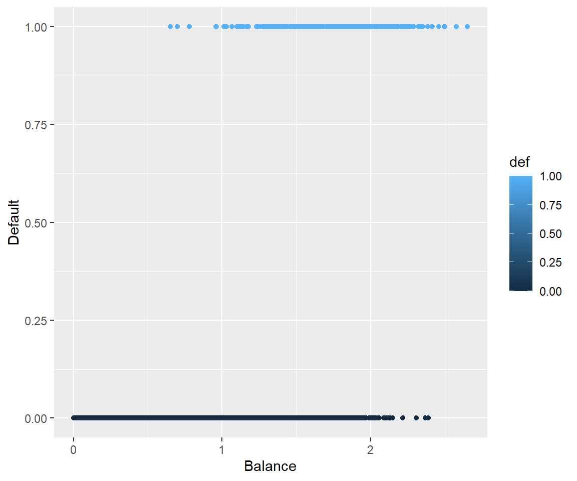

5.3.4 Why Not Linear Regression

We could use standard linear regression to model \(p(\text{Balance}) = p(x)\). The line on this plot represents the estimated probability of defaulting.

def.plot.lm <- ggplot(Default, aes(x = balance, y = def, color = def)) + geom_point()+
  xlab("Balance") + ylab("Default") +
  geom_smooth(method = 'lm')

def.plot.lm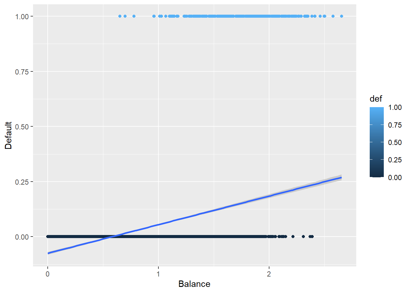

Can you think of any issues with this? Think about possible values of \(p(x)\).

5.3.5 Plotting the Logistic Regression Curve

Here is the curve for a logistic regression.

def.plot.logit <- ggplot(Default, aes(x = balance, y = def, color = def)) + geom_point() +
  xlab("Balance") + ylab("Default") +
  geom_smooth(method = "glm", method.args = list(family = "binomial"))
  
def.plot.logit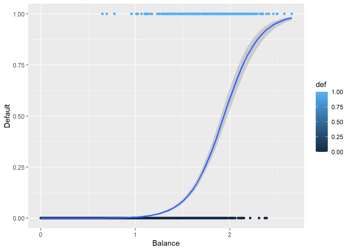

How does this compare to the previous plot?

5.4 The Logistic Model in GLM

Even though we are trying to model a \(p(x)\), we are trying to model a mean.

What is the mean or Expected Values of a binomial random variable \(Y|x \sim\) Binomial\((1, p(x))\)?

Before we get into the link function, lets look at the function that models \(p(x)\)

\[ p(x) = \dfrac{e^{\beta_0 + \beta_1x}}{1 + e^{\beta_0 + \beta_1x}} \]

The link functions for Logistic Regression is the logit function which is

\[ \text{logit}(x) = \log\left(\frac{m}{1-m}\right) \text{ where } 0<x<1 \]

Which for \(\mu_{y|x} = p(x)\) is

\[ \log\left( \frac{p(x)}{1-p(x)} \right) = \beta_0 + \beta_1 x \]

• Notice that now we have a linear function of the coefficients.

• Something to pay attention to: When we are interpreting the coefficients, we are talking about how the log odds change.

• The coefficients tell us what the percentage increase of the odds ratio would be.

\[ \text{Odds} = \frac{p(x)}{1-p(x)} \]

5.4.1 Estimating The Coefficients: glm function

The function that is used for GLMs in R is the glm function.

glm(formula, family = gaussian, data)

• formula: the linear formula you are using when the link function is applied to \(\mu(vx)\). This has same format as lm, e.g, y ~ x

• family: the distribution of \(Y\) which in logistic regression is binomial

• data: the dataframe… as has been the case before.

5.4.2 GLM Function on Default Data

default.fit <- glm(def ~ balance, family = binomial, data = Default)

summary(default.fit)

Call:
glm(formula = def ~ balance, family = binomial, data = Default)

Coefficients:
            Estimate Std. Error z value Pr(>|z|)    
(Intercept) -10.6513     0.3612  -29.49   <2e-16 ***
balance       5.4989     0.2204   24.95   <2e-16 ***
---
Signif. codes:  0 '***' 0.001 '**' 0.01 '*' 0.05 '.' 0.1 ' ' 1

(Dispersion parameter for binomial family taken to be 1)

    Null deviance: 2920.6  on 9999  degrees of freedom
Residual deviance: 1596.5  on 9998  degrees of freedom
AIC: 1600.5

Number of Fisher Scoring iterations: 8

5.4.3 Default Predictions

“Predictions” in GLM models get a bit trickier than previously.

• We can predict in terms of the linear response, \(g(\mu(x))\), e.g., log odds in logistic regression.

• Or we can predict in terms of the actual response variable, e.g., \(p(x)\) in logistic regression.

\[ \log\left(\frac{\widehat{p}(x)}{1-\widehat{p}(x)}\right) = -10.6513 + 5.4090x \]

Which may not be very useful in application.

log

So for someone with a credict balance of 1000 dollars, we would predict that their probability of defaulting is

\[ \widehat{p}(x) = \frac{e^{-10.6513 + 5.4090\cdot 1}}{1 + e^{-10.6513 + 5.4090 \cdot 1}} = 0.00526 \]

And for someone with a credit balance of 2000 dollars, our prediction probability for defaulting is

\[ \widehat{p}(x) = \frac{e^{-10.6513 + 5.4090\cdot 2}}{1 + e^{-10.6513 + 5.4090 \cdot 2}} = 0.54158 \]

5.5 Interpreting coefficients

Because of what’s going on in logistic regression, we have forms for our model:

1. The linear form which is for predicting log-odds.
2. Odds ratios which is the exponentiated form of the model, i.e., \(e^{\beta_0 + \beta_1x}\).

• Then, we look at odds increasing (positive \(\beta_1\)) or decreasing (negative \(\beta_1\)) by \(e^{\beta_1}\) times.

3. Probabilities which are of the form \(\frac{e^{\beta_0 + \beta_1x}}{1 + e^{\beta_0 + \beta_1x}}\).

• Then \(\beta_1\) means… Nothing really intuitive.
• You just say \(\beta_1\) indicates increasing or decreasing probability respective of whether \(\beta_1\) is postive or negative.

Honestly, GLMs are where interpretations get left behind because the link functions screw with our ability to make sense of the math.

We will address this later with looking at “marginal effects”

5.6 Predict Function for GLMS

We can compute our predictions by hand but, that’s not super efficient. We can infact use the predict function on glm objects just like we did with lm objects.

With GLMs, our predict function now takes the form:

predict(glm.model, newdata, type)

• glm.model is the glm object you created to model the data.
• newdata is the data frame with values of your predictor variables you want predictions for. If no argument is given (or its incorrectly formatted) you will get the fitted values for your training data.
• type chooses which form of prediction you want.
  • type = "link" (the default option) gives the predictions for the link function, i.e, the linear function of the GLM. So for logistic regression it will spit out the predicted values of the log odds.
  • type = "response" gives the prediction in terms of your response variable. For Logistic Regression, this is the predicted probabilities.
  • type = "terms" returns a matrix giving the fitted values of each term in the model formula on the linear predictor scale. (idk)

5.6.1 Using predict on Default Data

Let’s get predictions from the logistic regression model that’s been created.

predict(default.fit, newdata = data.frame(balance = c(1,2)), type = "link")

         1          2 
-5.1524137  0.3465032 

predict(default.fit, newdata = data.frame(balance = c(1,2)), type = "response")

          1           2 
0.005752145 0.585769370 

5.6.2 Classifying Predictions

If we are looking at the log odds ratio, we will classify an observation as a \(\widehat{Y}= 1\) if the log odds is non-negative.

Default$pred.link <- predict(default.fit)
Default$pred.class1 <-as.factor(ifelse(Default$pred.link >=0, 1, 0))

Or we can classify based off the predicted probabilities, i.e., \(\widehat{Y} = 1\) if \(\widehat{p}(x) \geq 0.5\).

Default$pred.response <- predict(default.fit, type = "response")
Default$pred.class2 <-as.factor(ifelse(Default$pred.response >=0.5, 1, 0))

Which will produce identical classifications.

sum(Default$pred.class1 != Default$pred.class2)

[1] 0

5.6.3 Assessing Model Accuracy

We can assess the accuracy of the model using a confusion matrix using the confusionMatrix function, which is part of the caret package.

• Note that this will require you to install the e1071 package (which I can’t fathom why they would do it this way…).

confusionMatrix(Predicted, Actual)

confusionMatrix(Default$pred.class1, as.factor(Default$def))

Confusion Matrix and Statistics

          Reference
Prediction    0    1
         0 9625  233
         1   42  100
                                          
               Accuracy : 0.9725          
                 95% CI : (0.9691, 0.9756)
    No Information Rate : 0.9667          
    P-Value [Acc > NIR] : 0.0004973       
                                          
                  Kappa : 0.4093          
                                          
 Mcnemar's Test P-Value : < 2.2e-16       
                                          
            Sensitivity : 0.9957          
            Specificity : 0.3003          
         Pos Pred Value : 0.9764          
         Neg Pred Value : 0.7042          
             Prevalence : 0.9667          
         Detection Rate : 0.9625          
   Detection Prevalence : 0.9858          
      Balanced Accuracy : 0.6480          
                                          
       'Positive' Class : 0               
                                          

5.7 Categorical Predictors

Having categorical variables and including multiple predictors is pretty easy. It’s just like with standard linear regression.

Let’s look at the model that just uses the student variable to predict the probability of defaulting.

default.fit2 <- glm(def ~ student,
                    family = binomial,
                    data = Default)

summary(default.fit2)

Call:
glm(formula = def ~ student, family = binomial, data = Default)

Coefficients:
            Estimate Std. Error z value Pr(>|z|)    
(Intercept) -3.50413    0.07071  -49.55  < 2e-16 ***
studentYes   0.40489    0.11502    3.52 0.000431 ***
---
Signif. codes:  0 '***' 0.001 '**' 0.01 '*' 0.05 '.' 0.1 ' ' 1

(Dispersion parameter for binomial family taken to be 1)

    Null deviance: 2920.6  on 9999  degrees of freedom
Residual deviance: 2908.7  on 9998  degrees of freedom
AIC: 2912.7

Number of Fisher Scoring iterations: 6

predict(default.fit2, 
        newdata = data.frame(student = c("Yes", 
                                         "No")), 
        type = "response")

         1          2 
0.04313859 0.02919501 

Would student status by itself be useful for classifying individuals as defaulting or no?

5.8 Multiple Predictors

Similarly (Why isn’t there an ‘i’ in that?) to categorical predictors we can easily include multiple predictor variables. Why? Because with the link function, we are just doing linear regression.

\[ p_{y|x} = \dfrac{e^{\beta_0 + \beta_1x_1 + \beta_2x_2 \dots + \beta_px_p}}{1 + e^{\beta_0 + \beta_1x_1 + \beta_2x_2 \dots + \beta_px_p}} \]

The link functions is still the same.

\[ \text{logit}(m) = \log\left(\frac{m}{1-m}\right) \text{ where } 0<x<1 \]

Which for \(\mu_{y|x} = p_{y|x}\) is

\[ \log\left( \frac{p_{y|x}}{1-p_{y|x}} \right) = \beta_0 + \beta_1x_1 + \beta_2x_2 \dots + \beta_px_p \]

5.8.1 Multiple Predictors in Default Data

Lets look at how the model does with using balance, income, and student as the predictor variables.

default.fit3 <- glm(def ~ balance + income + student, family = binomial, data = Default)

summary(default.fit3)

Call:
glm(formula = def ~ balance + income + student, family = binomial, 
    data = Default)

Coefficients:
              Estimate Std. Error z value Pr(>|z|)    
(Intercept) -10.869045   0.492256 -22.080  < 2e-16 ***
balance       5.736505   0.231895  24.738  < 2e-16 ***
income        0.003033   0.008203   0.370  0.71152    
studentYes   -0.646776   0.236253  -2.738  0.00619 ** 
---
Signif. codes:  0 '***' 0.001 '**' 0.01 '*' 0.05 '.' 0.1 ' ' 1

(Dispersion parameter for binomial family taken to be 1)

    Null deviance: 2920.6  on 9999  degrees of freedom
Residual deviance: 1571.5  on 9996  degrees of freedom
AIC: 1579.5

Number of Fisher Scoring iterations: 8

predict(default.fit3, 
        newdata = data.frame(balance = c(1,2), 
                             student = c("Yes",
                                         "No"), 
                             income=40),
        type = "response")

          1           2 
0.003477432 0.673773774 

predict(default.fit3, 
        newdata = data.frame(balance = c(1), 
                             student = c("Yes", 
                                         "No"), 
                             income=c(10, 50)),
        type = "response")

          1           2 
0.003175906 0.006821253 

5.9 Logistic Regression Diagnostics and Model Selection

Things are a bit different in GLMs. There is no assumption of normality and the definition of a residual is much more ambiguous.

• We verify the linearity assumption, i.e., \(g(\mu_{y|x})\) is linearly related to the predictors. (NOT \(\mu_{y|x}\)).
  • This one is a bit difficult to tease out.
• We check multicollinearty/VIF like before.
• Assess for influential observations.

5.10 Data: Do you have mesothelioma? If so call \(<ATTORNEY>\) at \(<PHONE NUMBER>\) now.

5.10.1 Data description

From UCI Machine Learning Repository: https://archive.ics.uci.edu/ml/datasets/Mesothelioma%C3%A2%E2%82%AC%E2%84%A2s+disease+data+set+

This data was prepared by; >Abdullah Cetin Tanrikulu from Dicle University, Faculty of Medicine, Department of Chest Diseases, 21100 Diyarbakir, Turkey e-mail:cetintanrikulu ‘@’ hotmail.com Orhan Er from Bozok University, Faculty of Engineering, Department of Electrical and Electronics Eng., 66200 Yozgat, Turkey e-mail:orhan.er@bozok.edu.tr

In order to perform the research reported, the patient’s hospital reports from Dicle University, Faculty of Medicine’s were used in this work. One of the special characteristics of this diagnosis study is to use the real dataset taking from patient reports from this hospital. Three hundred and twenty-four MM patient data were diagnosed and treated. These data were investigated retrospectively and analysed files.

In the dataset, all samples have 34 features because it is more effective than other factors subsets by doctor’s guidance. These features are; age, gender, city, asbestos exposure, type of MM, duration of asbestos exposure, diagnosis method, keep side, cytology, duration of symptoms, dyspnoea, ache on chest, weakness, habit of cigarette, performance status, White Blood cell count (WBC), hemoglobin (HGB), platelet count (PLT), sedimentation, blood lactic dehydrogenise (LDH), Alkaline phosphatise (ALP), total protein, albumin, glucose, pleural lactic dehydrogenise, pleural protein, pleural albumin, pleural glucose, dead or not, pleural effusion, pleural thickness on tomography, pleural level of acidity (pH), C-reactive protein (CRP), class of diagnosis. Diagnostic tests of each patient were recorded.

5.11 Model Selection

There are a lot of variables in the data…AND I don’t have a code book for what some of the stuff means.

What do I do?

meso <- read_csv(here::here("datasets","Meso.csv"))
spec(meso)

cols(
  age = col_double(),
  gender = col_double(),
  city = col_double(),
  asbExposure = col_double(),
  asbDuration = col_double(),
  dxMethod = col_double(),
  cytology = col_double(),
  symDuration = col_double(),
  dyspnoea = col_double(),
  chestAche = col_double(),
  weakness = col_double(),
  smoke = col_double(),
  perfStatus = col_double(),
  WB = col_double(),
  WBC = col_double(),
  HGB = col_double(),
  PLT = col_double(),
  sedimentation = col_double(),
  LDH = col_double(),
  ALP = col_double(),
  protein = col_double(),
  albumin = col_double(),
  glucose = col_double(),
  PLD = col_double(),
  PP = col_double(),
  PA = col_double(),
  PG = col_double(),
  dead = col_double(),
  PE = col_double(),
  PTH = col_double(),
  PLA = col_double(),
  CRP = col_double(),
  dx = col_double()
)

5.11.1 Step one: Assess your goal and how you get there.

The goal will be to predict the probability of the subject having mesothelioma:

• dx is 1 for mesothelioma, 0 if “healthy”
• I want to do this for people that are ALIVE. And I want to do it based on the characteristics of the person
  • The dead variable is therefore useless to me, I can get rid of it.
  • dxMethod doesn’t seem useful for my goal by its name either.
  • I’m suspicious of cytology since it may be whether a specific type of test is used. That would not be helpful in actually predicting if someone has mesothelioma based on the attributes of that person.
• There are many categorical variables that I don’t know how they are coded.
  • city, smoke, perfStatus
  • If I can’t assess how they contribute to the model, I’m not going to use them.
  • I don’t know how to measure those variables for future use of the model.
  • Also, as a statistician, I can’t give meaningful results if I don’t have information about a variable.

meso2 <- meso %>%
  select(-dead, -dxMethod, -cytology, -city, -smoke, -perfStatus)

That still leaves of with 24 variables…

5.11.2 Variance Inflaction Factors are still here

Let’s start with the full model.

fullModel <- glm(dx ~ ., binomial, meso2)

Now get the VIFs (courtesy of ’car library)

vif(fullModel)

          age        gender   asbExposure   asbDuration   symDuration 
     1.623728      1.097621      2.719456      3.482200      1.141027 
     dyspnoea     chestAche      weakness            WB           WBC 
     1.094622      1.062902      1.220221      1.119346      1.124898 
          HGB           PLT sedimentation           LDH           ALP 
     1.157734      1.886302      1.135334      1.870804      1.247170 
      protein       albumin       glucose           PLD            PP 
     1.336606      1.413671      1.102442      1.250738      7.939269 
           PA            PG            PE           PTH           PLA 
     7.117496      2.344206      2.351430      1.705495      1.878006 
          CRP 
     1.565218 

• The criteria is about the same as before:

• If there are any VIFs greater than 5, investigate.

• If there are more than a few (no hard rule to give) in the 2 to 5 range or things seem weird, investigate.

• What strikes me is absExposure and absDuration.

  • These are whether someone has been exposed, and if so, how long were they exposed in days.
  • They are NOT independent of each other.
  • There are things to consider which one is wisest to remove.
  • asbDuration contains information about both, so maybe that’s best.

• That leaves us mainly with PP (pleural protein?) and PA (pleural albumin?)

  • They seem to be fairly correlated with each other.
  • I have no idea what is more important (maybe you would!) so I’m going to take PP out.
  • A less arbitrary option may be to try two models, one with each missing, and see how well they fit/perform.

ggplot(meso2, aes(x = PP, y = PA)) +
  geom_point()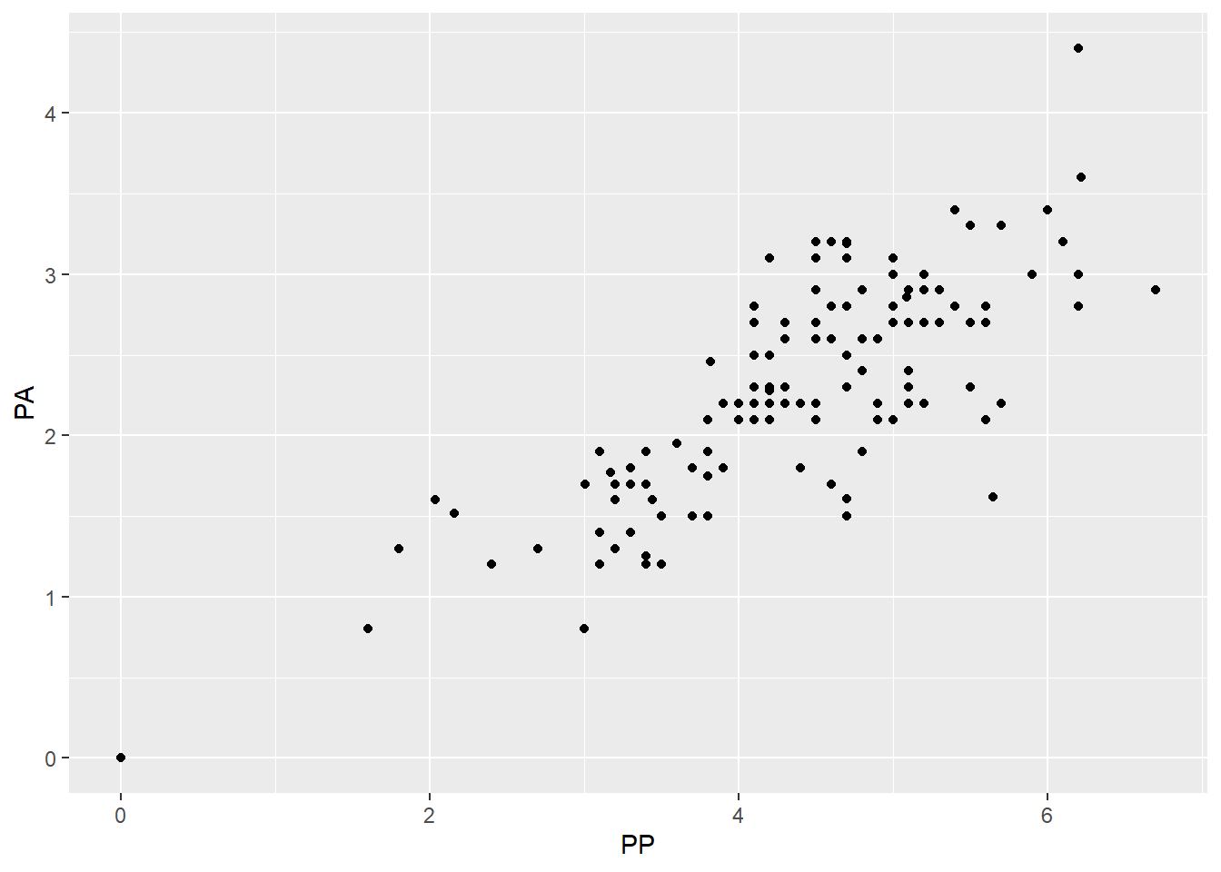

5.11.3 Check after removing variables

So lets cut the variables down a bit more and check how things are doing.

meso3 <- meso2 %>%
  select(-PP, -asbExposure)

fullModel2 <- glm(dx ~ ., binomial, meso3)

summary(fullModel2)

Call:
glm(formula = dx ~ ., family = binomial, data = meso3)

Coefficients:
                Estimate Std. Error z value Pr(>|z|)   
(Intercept)    1.227e+00  1.944e+00   0.631  0.52779   
age           -4.656e-02  1.472e-02  -3.163  0.00156 **
gender        -7.519e-01  2.735e-01  -2.749  0.00597 **
asbDuration    2.945e-02  1.059e-02   2.781  0.00541 **
symDuration    5.788e-02  2.902e-02   1.994  0.04611 * 
dyspnoea      -2.021e-02  3.484e-01  -0.058  0.95375   
chestAche     -2.540e-01  2.830e-01  -0.898  0.36939   
weakness       3.429e-01  2.964e-01   1.157  0.24726   
WB            -1.577e-05  3.982e-05  -0.396  0.69201   
WBC           -6.393e-02  4.185e-02  -1.528  0.12655   
HGB            3.258e-01  2.844e-01   1.146  0.25195   
PLT           -2.201e-03  1.140e-03  -1.931  0.05349 . 
sedimentation  4.768e-03  6.457e-03   0.738  0.46024   
LDH            4.156e-04  9.604e-04   0.433  0.66522   
ALP           -8.684e-04  4.290e-03  -0.202  0.83961   
protein        7.299e-02  1.800e-01   0.405  0.68512   
albumin        6.421e-02  2.442e-01   0.263  0.79262   
glucose        2.416e-03  3.496e-03   0.691  0.48940   
PLD           -1.459e-04  3.582e-04  -0.407  0.68367   
PA            -2.819e-01  1.862e-01  -1.514  0.12996   
PG            -8.418e-03  7.333e-03  -1.148  0.25097   
PE             1.416e-01  5.414e-01   0.262  0.79366   
PTH            2.249e-01  3.475e-01   0.647  0.51747   
PLA           -7.894e-01  3.567e-01  -2.213  0.02689 * 
CRP            1.226e-02  7.395e-03   1.658  0.09730 . 
---
Signif. codes:  0 '***' 0.001 '**' 0.01 '*' 0.05 '.' 0.1 ' ' 1

(Dispersion parameter for binomial family taken to be 1)

    Null deviance: 393.79  on 323  degrees of freedom
Residual deviance: 348.20  on 299  degrees of freedom
AIC: 398.2

Number of Fisher Scoring iterations: 5

vif(fullModel2)

          age        gender   asbDuration   symDuration      dyspnoea 
     1.434130      1.088232      1.487264      1.129502      1.094376 
    chestAche      weakness            WB           WBC           HGB 
     1.045581      1.178690      1.115586      1.096017      1.157860 
          PLT sedimentation           LDH           ALP       protein 
     1.858685      1.140208      1.871628      1.230647      1.306394 
      albumin       glucose           PLD            PA            PG 
     1.344529      1.098984      1.235294      1.800686      2.337586 
           PE           PTH           PLA           CRP 
     2.122909      1.701094      1.857195      1.558289 

Everything is way better in terms of VIF so that’s a good first step I’d say.

5.12 Residual Diagnostics

5.12.1 Review

Assessing the residuals is a bit difficult here, originally it was pretty simple.

\[e_i = \text{observed} - \text{predicted} = y_i - \hat y_i\]

And then there are standardized residuals and studentized residuals (which get called standardized residuals because someone was sadistic).

\[e^*_i = \frac{y_i - \hat y_i}{\sqrt{MSE}} \qquad \text{or} \qquad e^*_i = \frac{y_i - \hat y_i}{\sqrt{MSE(1 - h_i)}}\]

• Both have the same objective: set the residuals on the same scale no matter what model you’re examining.
• Standardized/Studentized Residuals greater than 3 are considered outl;iers and the corresponding data point should be investigated.
• Studentized residuals (the right hand-side version) are calculated in such a way that they try to account for over-fitting of the model to the data by pretending that observation is not in the data.
• It is my impression (and opinion) that Studentized should be preferred.

5.12.2 Residuals in GLMs

Residuals follow the same form.

\[e_i = \text{observed} - \text{predicted} = y_i - \hat y_i\]

The general form for a standardized residual is about the same:

\[e_i = \frac{y_i - \hat y_i}{s(\hat y_i)}\]

and \(s(\hat y_i)\) is the variability of our estimate.

• In GLMs it is often the case, \(s(\hat y_i)\) is not constant by default, i.e., the variability of the predictions is not constant.
• Dependent on our model, the way to calulate \(s(\hat y_i)\) differs.

5.12.3 Pearson Residuals

We have to account for the fact that our predictions are probabiliies in logistic regression.

\[\hat y_i = \widehat P(y_i = 1| x) = \widehat p_i(x_i)\]

We are dealing with the binomial distribution so the formula for the variability of the predicted probability is:

\[s(\hat y_i) = \sqrt{\widehat p_i(x_i)(1-\widehat p_i(x_i))}\]

Therefore the Pearson standardized residual is:

\[e_i = \frac{y_i - \widehat p_i(x_i)}{\sqrt{\widehat p_i(x_i)(1-\widehat p_i(x_i))}}\]

If you can group your predictions somehow in groups of size \(n_i\), then the pearson residual is

\[e_i = \frac{y_i - \widehat p_i(x_i)}{\sqrt{n_i\widehat p_i(x_i)(1-\widehat p_i(x_i))}}\]

5.12.4 Deviance residuals

There is something called a deviance residual, for which the formula is:

\[e^*_i = sign(y_i - \hat y_i)\sqrt{2 [ y_i \log(\frac{y_i}{\hat y_i}) + (n_i-y_i) \log(\frac{n_i-y_i}{n_i -\hat y_i}) ]}\]

• The formula is not very illuminating unless you have deeper theoretical knowledge.
• I have seen at least one person say this is “preferred”.
• I have also seen that examining them is about the same as examining the pearson residuals.
• An advantage here is that deviance residuals are universal and relate to some of the deeper structure of GLMs.

5.12.5 Autoplot maybe?

We can examine the residuals via autoplot and assess outliers as well..

autoplot(fullModel, which = c(1,2,4))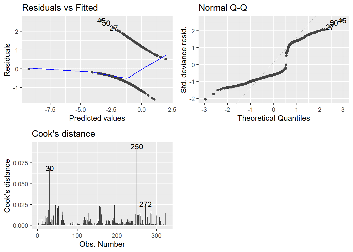

• Technically, these plots indicate that nothing is wrong.
  • There is a lot of intuition and theory type stuff for why I can say that.
  • That might be a whole more week’s worth of material, but we are cutting here.
  • Consider it a self study topic.
  • Hopefully, I’ve given enough of a seed of information for you to teach yourself more in depth modeling.
  • If you want to be good, the learning never ends.

Anyway, on to the plots.

• Top-left may not be familiar since our observed values are either zero or one.
• QQ plot looks weird because there is not a normal distribution to expect, necessarily.
• Cook’s distance is at least familiar.
  • 0.5 denotes a potentially problematic value.
  • 1 is the cutoff for an extreme outlier.
  • Some people say 4/n is a good cutoff… I have found no reason to back that up so far.
• Honestly I am still at a loss for how useful examination of the plots can be. GLMs can really mess with traditional methods.

5.12.6 DHARMa package for plotting residuals.

An experimental way of examining the residuals is available via the DHARMa package.

Florian Hartig (2021). DHARMa: Residual Diagnostics for Hierarchical (Multi-Level / Mixed) Regression Models. R package version 0.4.1. https://CRAN.R-project.org/package=DHARMa

• It tries to streamline the process and make it easier for non-experts to examine residuals via simulation.
• There are only a couple of functions you need to know.
  • simulateResiduals(model) which is stored as a variable.
  • plot(simRes) where simRes is the simulated residuals output variable.
• Because it runs simulations (repeated calculations), it may take a while to finish.

# install.packages('DHARMa')

library(DHARMa)

simRes <- simulateResiduals(fullModel)

plot(simRes)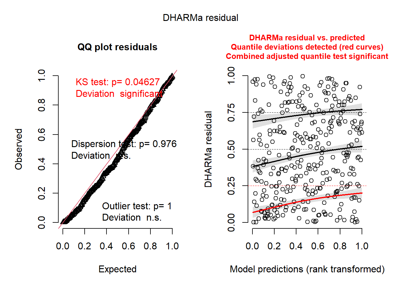

Notice the output basically tells you what may or may not be wrong. It’s as simple as that.

• The QQ Plot is NOT for normality.
  • BUT you still want to check if they follow a straight line.
  • The KS Test p-value is for the test of whether the data are following the correct distribution or not.
  • Small p-values mean there are problems with your model.
• Here everything seems ideal.
  • The QQ-Plot is a nearly straight line.
  • The residual plot on the right follows the pattern we’d want. Everything is centered at 0 and the spread is consistent.
• I cannot 100% recommend that this is all that you rely on, I am merely proposing a tool to get an overview of the situation.
• In reality there are a LOT of nuances to what’s going on, so be wary.
• As far as the relative simplicity of the models we look at, my guess is that this is fine to use.

5.13 Marginal Effects in Generalized Linear Models (GLMs)

When working with statistical models, especially complex ones like GLMs that include nonlinear components, interactions, or transformations, the raw parameter estimates (coefficients) can be difficult to interpret substantively. Marginal effects provide a solution by transforming these raw estimates into quantities that are easier for researchers and stakeholders to understand. The computations used here are useful beyond GLMs, as you will see later with ANOVA, but is essential when dealing with link functions.

5.13.1 What Are Marginal Effects?

Marginal effects are partial derivatives of the regression equation with respect to a predictor of interest. In simple terms, they tell us:

“If a predictor were to change from its observed value by a small amount, the marginal effect is the rate at which the prediction would change.”

5.13.1.1 Key Characteristics:

• They measure the instantaneous rate of change in the predicted outcome
• They are only defined for continuous predictors (not categorical ones)
• In economics and political science, they’re often called “marginal effects” where “marginal” refers to a small change

5.13.2 Why Are Marginal Effects Crucial for GLMs?

1. Nonlinear Relationships Unlike linear models where coefficients directly represent the change in Y for a unit change in X, GLMs involve:

• Link functions (e.g., logit, probit) that create nonlinear relationships
• Non-constant effects that vary depending on the values of other predictors

2. Scale Issues GLM coefficients are often on transformed scales:

• Logistic regression: Coefficients are in log-odds units
• Poisson regression: Coefficients are in log units

These scales are not intuitive for interpretation!

3. Interaction Effects When GLMs include interactions, the effect of one variable depends on the values of other variables, making simple coefficient interpretation inadequate.

5.13.3 Digging Deeper

Suppose you have a regression model predicting house prices:

\[\text{Price} = \beta_0 + \beta_1(\text{SquareFeet}) + \beta_2(\text{Bedrooms}) + \beta_3(\text{Age})\]

The marginal effect of square footage is simply \(\beta_1\) - it tells you how much the predicted price increases for each additional square foot, holding bedrooms and age constant.

For more complex models like logistic regression, the marginal effect isn’t constant. If you have:

\[P(\text{Success}) = \frac{1}{1 + e^{-(\beta_0 + \beta_1 X_1 + \beta_2 X_2)}}\]

The marginal effect of \(X_1\) is:

\[\frac{\partial P}{\partial X_1} = \beta_1 \times P \times (1-P)\]

This means the marginal effect depends on the current probability level and varies across observations.

5.14 Example: Why Raw Coefficients Can Mislead

Consider a logistic regression predicting whether a country has impartial institutions:

Coefficient for "Equal distribution" = 0.046

Problems with this raw coefficient:

• It’s in log-odds units (not intuitive)
• The actual effect depends on values of other predictors
• With interactions, the effect varies across different contexts

Marginal effect interpretation:

• “A one-unit increase in equality index increases the probability of impartial institutions by 0.54 percentage points (on average)”
• Much more meaningful for policy discussions!

5.15 Types of Marginal Effects

1. Average Marginal Effects (AME)

• Calculate marginal effect for each observation
• Take the average across all observations
• Interpretation: “On average, across all units in the sample…”

2. Marginal Effects at the Mean (MEM)

• Calculate marginal effect when all predictors are at their mean values
• Interpretation: “For a typical/average unit…”

3. Marginal Effects at Representative Values

• Calculate marginal effects at specific, substantively interesting values
• Interpretation: “For units with characteristics X, Y, Z…”

5.15.1 Computational Approach

Marginal effects are typically computed using:

1. Analytical derivatives (when feasible)
2. Numerical derivatives (more flexible, works with complex models)
   • Small perturbation method: [f(x + h) - f(x)] / h as h approaches 0

5.15.2 Practical Framework for Analysis

When computing marginal effects, consider these five key decisions:

1. Quantity: What do you want to measure? (predictions, comparisons, slopes)
2. Grid: At what values do you evaluate the effects?
3. Aggregation: Individual-level or averaged effects?
4. Uncertainty: How do you quantify standard errors?
5. Test: What hypotheses do you want to test?

5.15.3 Best Practices

5.15.3.1 Do:

• Always report marginal effects for GLMs alongside raw coefficients
• Specify the evaluation points clearly (at means, at representative values, etc.)
• Consider effect heterogeneity across different subgroups
• Visualize marginal effects to show how they vary across predictor values

5.15.3.2 Don’t:

• Interpret raw GLM coefficients as if they were from linear models
• Assume constant effects across all values of predictors
• Ignore interactions when computing marginal effects
• Forget confidence intervals for marginal effects

5.15.4 Another note on marginal effects

Marginal effects are not just a “nice-to-have” addition to GLM analysis—they are essential for proper interpretation. They bridge the gap between complex statistical models and substantive understanding, making research findings accessible to policymakers, stakeholders, and the broader scientific community.

“The goal is not just to fit complex models, but to extract meaningful insights that can inform decisions and advance knowledge.”

5.16 The Delta Method and Statistical Comparisons in GLMs

When working with GLMs, we often want to make comparisons between predictions or compute functions of parameters (like odds ratios, risk ratios, or marginal effects). However, these derived quantities don’t come with ready-made standard errors from our model output. The delta method provides a powerful mathematical technique to approximate the variance and standard errors of these complex functions.

5.16.1 What Is the Delta Method?

The delta method is a statistical technique used for approximating the variance and standard error of a function of a random variable based on the random variable’s own variance and standard error.

5.16.2 Mathematical Foundation:

For a function \(g(\theta)\) where \(\theta\) is our parameter estimate:

\[\text{Var}[g(\hat{\theta})] \approx [g'(\theta)]^2 \times \text{Var}(\hat{\theta})\]

Where:

• \(g'(\theta)\) is the derivative of function \(g\) with respect to \(\theta\)
• \(\hat{\theta}\) is our parameter estimate
• The approximation improves with larger sample sizes

5.16.3 Why Is the Delta Method Essential for GLM Comparisons?

1. Complex Transformations

GLMs often require us to compute:

• Predicted probabilities from logit coefficients
• Risk ratios from differences in probabilities
  
• Odds ratios from coefficient differences
• Marginal effects from partial derivatives

Each involves a nonlinear transformation of the original parameters.

2. Standard Error Propagation

When we transform parameters, we need to know:

• How uncertain our new quantity is
• Whether differences are statistically significant
• What the confidence intervals should be

Raw parameter standard errors don’t directly apply to transformed quantities!

3. Hypothesis Testing

To conduct meaningful tests on comparisons, we need:

• Standard errors for test statistics
• P-values for significance testing
• Confidence intervals for effect sizes

5.16.4 Practical Examples in GLMs

5.16.4.1 Example 1: Risk Difference from Logistic Regression

Scenario: Compare predicted probabilities between treatment and control groups.

\[\text{Raw coefficients: } \beta_0 = -1.2, \beta_1 = 0.8\]

Step 1: Compute predictions

• \(P(\text{Control}) = \text{logit}^{-1}(-1.2) = 0.23\)
• \(P(\text{Treatment}) = \text{logit}^{-1}(-1.2 + 0.8) = 0.38\)

Step 2: Compute risk difference

• \(\text{Risk Difference} = 0.38 - 0.23 = 0.15\)

Step 3: Apply delta method for standard error

• Need derivatives of \(\text{logit}^{-1}\) function
• Combine with variance-covariance matrix of \(\hat{\boldsymbol{\beta}}\)
• Result: \(\text{SE}(\text{Risk Difference}) \approx 0.04\)

5.16.4.2 Example 2: Odds Ratio Confidence Intervals

Raw coefficient: \(\beta_1 = 0.8\), \(\text{SE}(\beta_1) = 0.3\)

Transformation: \(\text{OR} = \exp(\beta_1) = \exp(0.8) = 2.23\)

Delta method application:

• \(g(\beta_1) = \exp(\beta_1)\)
• \(g'(\beta_1) = \exp(\beta_1)\)
• \(\text{Var}[\text{OR}] \approx [\exp(0.8)]^2 \times (0.3)^2 = (2.23)^2 \times 0.09 \approx 0.45\)
• \(\text{SE}(\text{OR}) \approx 0.67\)

95% CI: \(2.23 \pm 1.96 \times 0.67 = [0.92, 3.54]\)

5.16.5 Advantages of the Delta Method

1. Computational Efficiency

• Fast calculation compared to bootstrap methods
• Analytical solution when derivatives are available
• Scales well with large datasets

2. Theoretical Foundation

• Well-established mathematical basis
• Asymptotically correct (improves with sample size)
• Widely accepted in statistical literature

3. Flexibility

• Works with any differentiable function
• Handles multivariate transformations
• Supports complex hypothesis tests

5.16.6 Limitations and Considerations

1. Asymptotic Approximation

• May be inaccurate in small samples
• Assumes normality of the derived quantity
• Linear approximation of nonlinear functions

2. Derivative Requirements

• Function must be differentiable
• Numerical derivatives may introduce error
• Complex functions can be computationally challenging

3. Alternative Methods When delta method is inadequate, consider:

• Bootstrap methods for small samples
• Simulation-based inference for complex functions
• Exact methods when available

5.16.7 The Delta Method in Practice

5.16.7.1 Computational Steps:

1. Identify the transformation: What function \(g(\theta)\) are you computing?

2. Compute derivatives: Find \(g'(\theta)\) analytically or numerically

3. Extract variance-covariance matrix: Get \(\text{Var}(\hat{\theta})\) from your model

4. Apply the formula: \(\text{Var}[g(\hat{\theta})] \approx [g'(\theta)]^2 \times \text{Var}(\hat{\theta})\)

5. Construct inference: Use \(\text{SE} = \sqrt{\text{Var}[g(\hat{\theta})]}\) for tests and CIs

5.16.8 Modern Implementation:

• Automated in software: Most packages handle this behind the scenes
• Numerical derivatives: Software computes derivatives automatically
• User-friendly: Focus on specifying comparisons, not mathematical details

5.16.9 Multivariate Delta Method

For functions of multiple parameters \(g(\theta_1, \theta_2, \ldots, \theta_k)\):

\[\text{Var}[g(\hat{\boldsymbol{\theta}})] \approx \nabla g(\boldsymbol{\theta})^T \boldsymbol{\Sigma} \nabla g(\boldsymbol{\theta})\]

Where:

• \(\nabla g(\boldsymbol{\theta})\) is the gradient vector of partial derivatives
• \(\boldsymbol{\Sigma}\) is the variance-covariance matrix of \(\hat{\boldsymbol{\theta}}\)

5.16.10 Best Practices

Do:

• Use delta method as default for GLM comparisons
• Check assumptions (large sample, smooth functions)
• Compare with alternatives when in doubt (e.g., bootstrap)
• Report methodology in your methods section

Don’t:

• Assume perfect accuracy in small samples
• Ignore numerical precision issues
• Apply to non-differentiable functions
• Forget about multiple testing corrections

5.16.11 Example: Hypothesis Testing with Delta Method

Research Question: “Is the risk difference between treatment and control significantly different from 0.1?”

# Delta method automatically applied
avg_comparisons(model, 
                variables = "treatment",
                hypothesis = 0.1)  # Test H₀: Risk Difference = 0.1

Output:

Estimate  Std.Error  z    Pr(>|z|)  
0.15      0.04       1.25  0.211     

Interpretation: Cannot reject \(H_0\) that risk difference equals 0.1 (\(p = 0.211\)).

5.16.12 Common Delta Method Applications in GLMs

1. Logistic Regression

• Predicted probabilities: \(g(\boldsymbol{x}^T\hat{\boldsymbol{\beta}}) = \frac{1}{1 + \exp(-\boldsymbol{x}^T\hat{\boldsymbol{\beta}})}\)
• Odds ratios: \(g(\hat{\beta_j}) = \exp(\hat{\beta_j})\)
• Risk differences: \(g(\hat{\boldsymbol{\beta}}) = P(Y=1|\boldsymbol{x_1}) - P(Y=1|\boldsymbol{x_0})\)

2. Poisson Regression

• Rate ratios: \(g(\hat{\beta_j}) = \exp(\hat{\beta_j})\)
• Predicted counts: \(g(\boldsymbol{x}^T\hat{\boldsymbol{\beta}}) = \exp(\boldsymbol{x}^T\hat{\boldsymbol{\beta}})\)

3. Marginal Effects

• Partial derivatives: \(g(\hat{\boldsymbol{\beta}}) = \frac{\partial E[Y|\boldsymbol{x}]}{\partial x_j}\)

5.16.13 Conclusion

The delta method is the workhorse behind most statistical comparisons in GLMs. While users rarely need to implement it manually, understanding its principles helps us:

• Appreciate the uncertainty in our derived quantities
• Make informed decisions about when standard methods are appropriate
  
• Recognize limitations and when alternative approaches are needed
• Interpret software output with greater confidence

“The delta method transforms the complex problem of uncertainty quantification for functions of parameters into a manageable approximation that enables robust statistical inference.”

Key Takeaway: Every time you see a standard error for a marginal effect, predicted probability, or risk ratio from a GLM, the delta method is likely working behind the scenes to make that inference possible.

5.17 Custom Hypothesis Testing with Marginal Effects: Beyond Null Hypothesis Testing

Traditional statistical testing focuses on rejecting null hypotheses (typically \(H_0: \theta = 0\)), but this approach has limitations. In many research contexts, we want to ask more nuanced questions: “Are two treatments practically equivalent?” or “Is an effect meaningfully different from a specific threshold?” Custom hypothesis testing with marginal effects, including equivalence testing like TOST, provides powerful tools for these sophisticated research questions.

5.17.1 Beyond Traditional Null Hypothesis Testing

5.17.1.1 Problems with Traditional Approach:

• Absence of evidence ≠ evidence of absence
• Focus on rejecting \(H_0: \theta = 0\) may not match research goals

5.17.1.2 Custom Hypotheses Enable:

• Testing specific effect sizes of theoretical interest
• Establishing practical equivalence between treatments
• Comparing effects across subgroups
• Testing complex relationships between multiple parameters

5.17.2 Equivalence Testing: The TOST Procedure

Two One-Sided Tests (TOST) is designed to establish statistical equivalence or show that a meaningful difference does not exist.

5.17.2.1 Core Logic:

Instead of testing \(H_0: \theta = 0\), we test:

\[H_0: |\theta| \geq \Delta \quad \text{vs.} \quad H_1: |\theta| < \Delta\]

Where \(\Delta\) is the equivalence margin (the largest difference we consider practically unimportant).

5.17.3 TOST Implementation:

TOST involves two simultaneous one-sided tests:

1. Lower bound test: \(H_{01}: \theta \leq -\Delta\) vs. \(H_{11}: \theta > -\Delta\)
2. Upper bound test: \(H_{02}: \theta \geq +\Delta\) vs. \(H_{12}: \theta < +\Delta\)

Equivalence conclusion: Reject both \(H_{01}\) and \(H_{02}\) (i.e., \(p_{\text{TOST}} = \max(p_1, p_2) < \alpha\))

5.17.4 Practical Applications in GLMs

5.17.4.1 Example 1: Treatment Equivalence in Clinical Research

Research Question: “Is the new treatment equivalent to the standard treatment in terms of success probability?”

Setup:

• Logistic regression predicting treatment success
• Equivalence margin: \(\Delta = 0.05\) (5 percentage points)
• Want to show \(|P(\text{New}) - P(\text{Standard})| < 0.05\)

# Compute risk difference with equivalence test
avg_comparisons(model, 
                variables = "treatment",
                equivalence = c(-0.05, 0.05))

Output:

Estimate  Std.Error  z     p(NonInf)  p(NonSup)  p(Equiv)
-0.02     0.015      -1.33  0.008      0.001      0.008

Interpretation:

• \(p(\text{Equiv}) = 0.008 < 0.05\) → Treatments are equivalent
• The risk difference is statistically contained within ±5 percentage points

5.17.4.2 Example 2: Dose-Response Threshold Testing

Research Question: “Is the marginal effect of drug dosage meaningfully different from 0.1 response units per mg?”

Custom hypothesis: \(H_0: \frac{\partial P}{\partial \text{dose}} = 0.1\)

# Test specific marginal effect value
avg_slopes(model, 
           variables = "dose",
           hypothesis = 0.1)

Output:

Estimate  Std.Error  z    Pr(>|z|)  
0.085     0.020      -0.75  0.454     

Interpretation: Cannot reject \(H_0\) that marginal effect equals 0.1 (\(p = 0.454\))

5.17.5 Advanced Custom Hypothesis Examples

1. Cross-Group Comparisons

Research Question: “Is the treatment effect larger for men than for women?”

\[H_0: \beta_{\text{treatment×male}} = 0 \quad \text{vs.} \quad H_1: \beta_{\text{treatment×male}} > 0\]

# Compare marginal effects across groups
avg_comparisons(model, 
                variables = "treatment",
                by = "gender",
                hypothesis = "pairwise")  # Tests: Male - Female

2. Ratio-Based Hypotheses

Research Question: “Is the treatment effect twice as large in the high-risk group?”

\[H_0: \frac{\text{Effect}_{\text{high-risk}}}{\text{Effect}_{\text{low-risk}}} = 2\]

# Using row-based hypothesis syntax
avg_comparisons(model,
                variables = "treatment", 
                by = "risk_group",
                hypothesis = "b1 = b2 * 2")  # b1 = high-risk, b2 = low-risk

3. Non-inferiority Testing

Research Question: “Is the new treatment at least 80% as effective as the standard?”

\[H_0: \frac{P(\text{New})}{P(\text{Standard})} \leq 0.8 \quad \text{vs.} \quad H_1: \frac{P(\text{New})}{P(\text{Standard})} > 0.8\]

# One-sided equivalence test
avg_comparisons(model,
                variables = "treatment",
                comparison = "ratio",
                hypothesis = 0.8,
                alternative = "greater")

5.17.6 Types of Custom Hypotheses

1. Point Hypotheses

• \(H_0: \theta = c\) for specific constant \(c\)
• Example: Testing if marginal effect equals a regulatory threshold

2. Equivalence Hypotheses

• \(H_0: |\theta| \geq \Delta\) vs. \(H_1: |\theta| < \Delta\)
• Example: Bioequivalence studies, non-inferiority trials

3. Superiority/Non-inferiority

• \(H_0: \theta \leq \Delta\) vs. \(H_1: \theta > \Delta\)
• Example: Showing new treatment is better by at least \(\Delta\)

4. Complex Functions

• \(H_0: f(\theta_1, \theta_2, \ldots) = c\)
• Example: Testing ratios, differences of differences, elasticities

5.17.7 Choosing Equivalence Margins

5.17.7.1 Considerations for \(\Delta\):

1. Clinical/Practical Significance

   • What difference would change practice?
   • Regulatory guidelines or professional standards

2. Statistical Power

   • Larger \(\Delta\) → easier to prove equivalence
   • Smaller \(\Delta\) → more stringent test

3. Context-Specific Factors

   • Cost considerations
   • Risk tolerance
   • Historical effect sizes

5.17.7.2 Common Approaches:

• Fraction of control effect: \(\Delta = 0.2 \times |\text{control effect}|\)
• Clinical minimally important difference
• Regulatory guidance (e.g., FDA bioequivalence: 80%-125%)

5.17.8 Implementation Best Practices

1. Pre-specify Hypotheses

# Define equivalence margins a priori
equivalence_margin <- 0.05

# Document rationale in analysis plan
# "5 percentage points chosen based on clinical judgment..."

2. Power Analysis

• Calculate required sample size for equivalence testing
• Equivalence tests typically need larger samples than superiority tests

3. Multiple Testing Corrections

# Adjust for multiple comparisons
avg_comparisons(model,
                variables = c("treatment1", "treatment2"),
                equivalence = c(-0.05, 0.05),
                p.adjust = "holm")

4. Sensitivity Analysis

# Test different equivalence margins
margins <- c(0.03, 0.05, 0.07)
results <- map(margins, ~avg_comparisons(model, equivalence = c(-.x, .x)))

5.17.9 Common Mistakes and Pitfalls

❌ Don’t Do:

• Interpret non-significant traditional test as evidence of equivalence
• Choose equivalence margins after seeing the data
• Ignore the direction of effects in one-sided tests
• Forget about clinical significance when setting \(\Delta\)

✅ Do:

• Pre-specify equivalence margins with scientific justification
• Report confidence intervals alongside test results
• Consider practical significance of the equivalence region
• Use appropriate sample sizes for desired power

5.17.10 Example: Complete Equivalence Analysis

Scenario: Comparing two educational interventions

# 1. Fit model
model <- glm(pass ~ intervention + covariates, 
             family = binomial, data = education_data)

# 2. Define equivalence margin (2 percentage points)
equiv_margin <- 0.02

# 3. Test equivalence
result <- avg_comparisons(model,
                         variables = "intervention",
                         equivalence = c(-equiv_margin, equiv_margin))

# 4. Interpret results
print(result)

Output:

Estimate  Std.Error  z     p(NonInf)  p(NonSup)  p(Equiv)  CI_low  CI_high
0.008     0.012      0.67   0.031      0.748      0.748     -0.015   0.031

Interpretation:

• Equivalence not established: \(p(\text{Equiv}) = 0.031 < 0.05\)
• The difference in pass rates is not statistically within ±2 percentage points
• 95% CI [-1.5%, 3.1%] not entirely contained within equivalence region

5.17.11 Conclusion

Custom hypothesis testing with marginal effects represents a paradigm shift from traditional “reject-the-null” thinking to more nuanced, question-driven inference. Equivalence testing, in particular, allows researchers to:

• Establish practical equivalence between treatments
• Make positive claims about similarity
• Answer clinically relevant questions about effect sizes
• Move beyond statistical significance to practical importance

“The goal isn’t just to reject null hypotheses, but to answer the specific scientific questions that motivated our research in the first place.”

Key Takeaway: When your research question is “Are these treatments equivalent?” or “Is this effect meaningfully different from X?”, traditional null hypothesis testing falls short. Custom hypotheses with equivalence testing provide the statistical framework to answer these practically important questions with appropriate rigor.