Plot Distribution of Standardized Mean Difference (SMD)

Creates consonance plots (confidence curves and/or consonance density functions) for standardized mean differences (SMDs), allowing visualization of uncertainty around effect size estimates.

Usage

plot_smd(
  d,
  df,
  lambda = NULL,
  sigma = NULL,
  smd_ci = c("t", "z", "goulet", "nct"),
  smd_label = "SMD",
  type = c("c", "cd"),
  levels = c(0.5, 0.9, 0.95, 0.999)
)

Arguments

d

Estimate of the standardized mean difference (Cohen's d, Hedges' g, etc.).

df

Degrees of freedom for the standardized mean difference.

lambda

The non-centrality parameter for the standardized mean difference. Required when smd_ci = "goulet".

sigma

The standard error for the standardized mean difference. Required when smd_ci is "t" or "z".

smd_ci

Method for calculating SMD confidence intervals:

"t": central t-distribution method
"z": normal distribution method
"goulet": Goulet-Pelletier method
"nct": noncentral t-distribution method (not currently supported)

smd_label

Label for the x-axis indicating the SMD measure (default: "SMD"). Common labels include "Cohen's d", "Hedges' g", or "Glass's delta".

type

Choose which plot(s) to create:

"c": consonance function only (p-values across potential parameter values)
"cd": consonance density function only (distribution of plausible parameter values)
c("c", "cd"): both plots together (default)

levels

Numeric vector of confidence levels to display (default: c(.5, .9, .95, .999)). These correspond to the confidence intervals shown on the plot.

Value

A ggplot2 object or plot grid from cowplot.

Details

Consonance plots provide a graphical representation of the full range of confidence intervals for standardized mean differences at different confidence levels. These plots help visualize the uncertainty around effect size estimates and go beyond the traditional approach of reporting only a single confidence interval (typically 95%).

The function creates two types of visualizations:

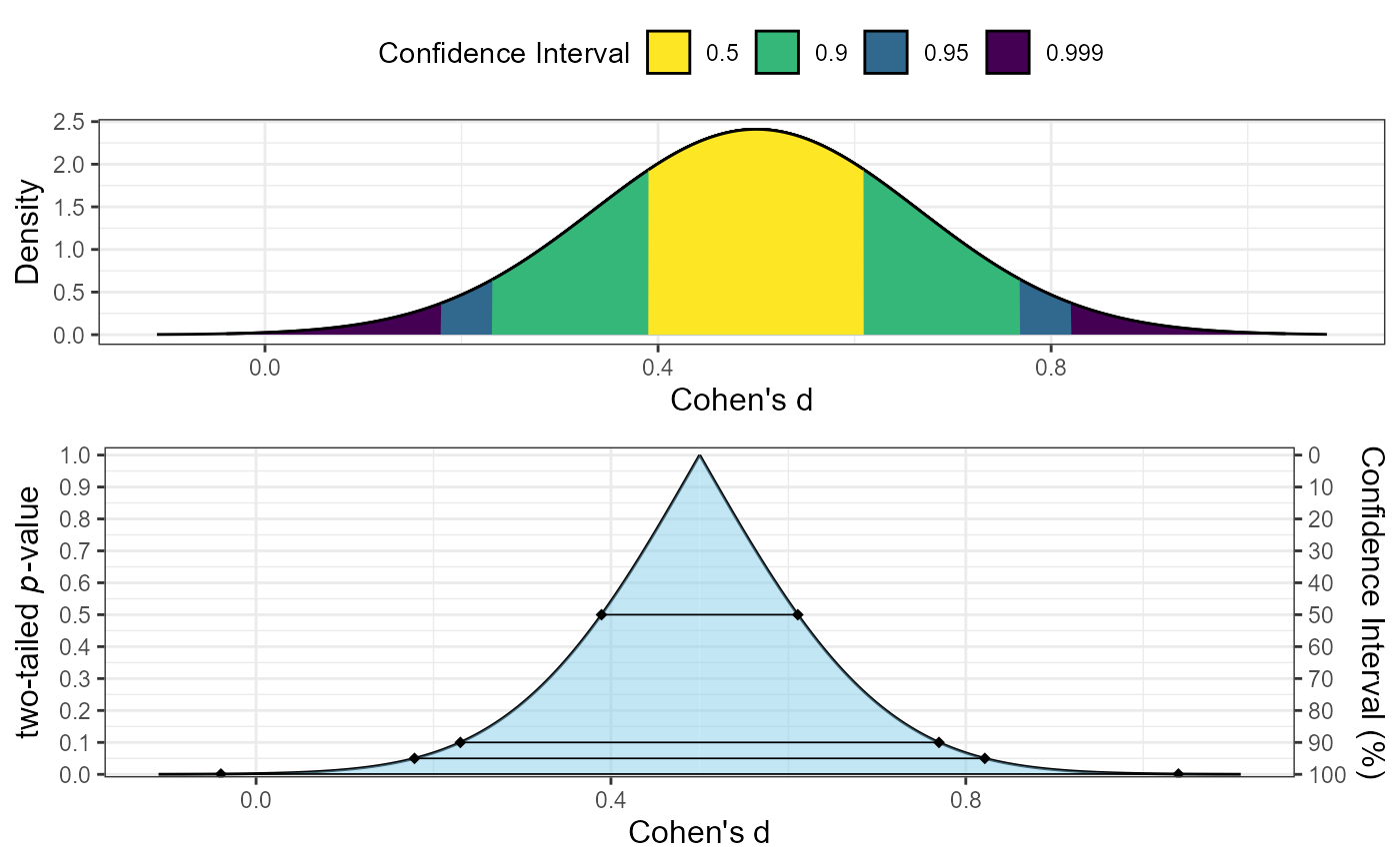
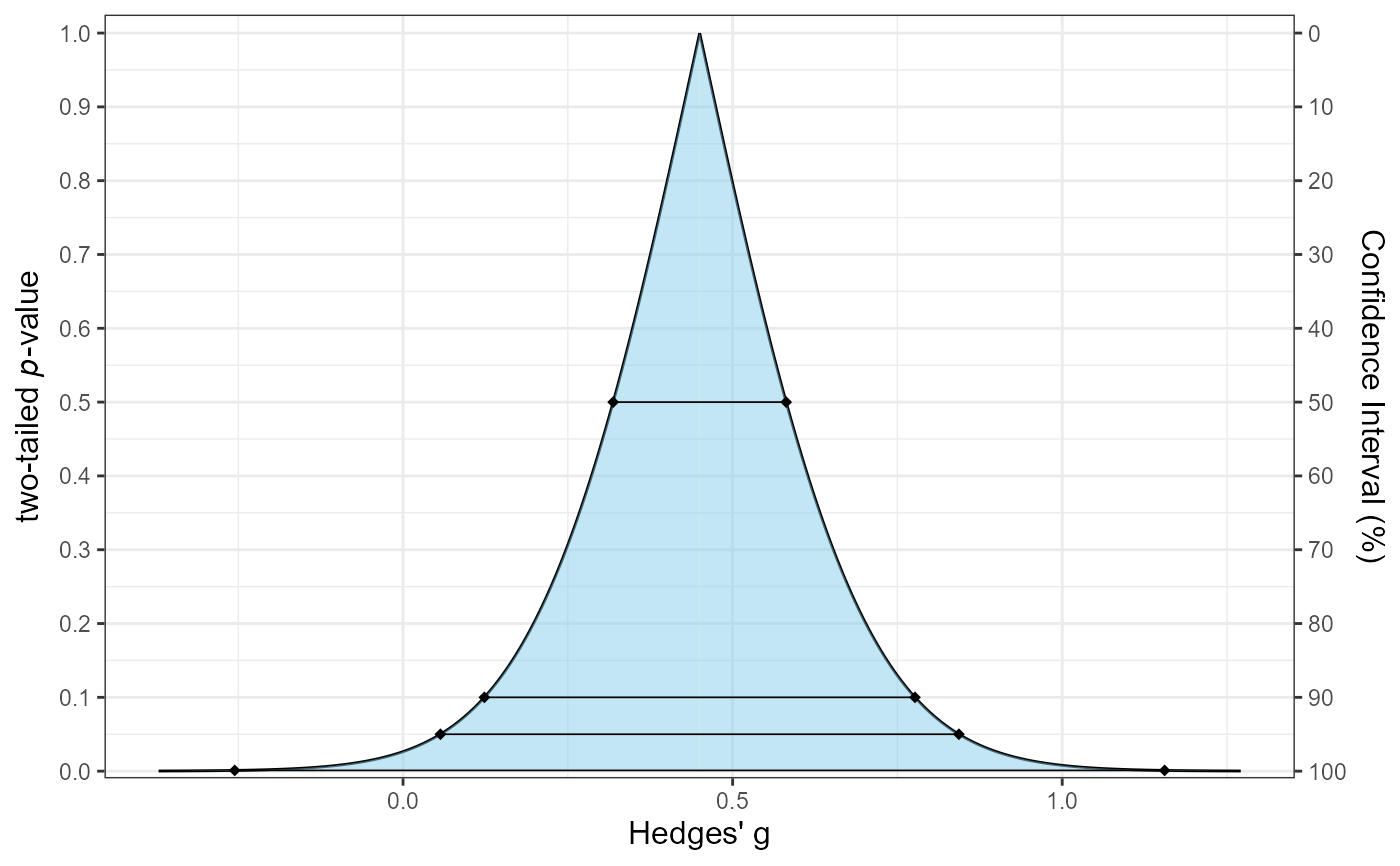
Consonance function ("c"): Shows how p-values change across different possible values of the SMD. The x-axis represents possible parameter values, and the y-axis represents the corresponding p-values from two-sided hypothesis tests.
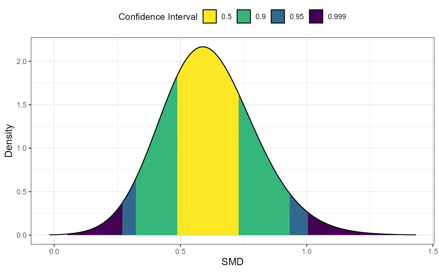
Consonance density ("cd"): Shows the distribution of plausible values for the SMD. This can be interpreted as showing where the "weight of evidence" is concentrated.

This function requires specific input parameters depending on the chosen confidence interval method:

For "goulet" method: d, df, and lambda must be provided
For "t" and "z" methods: d, df, and sigma must be provided
The "nct" method is not currently supported

The required parameters can typically be extracted from the results of functions like t_TOST(), smd_calc(), or from the smd component of these function results.

These plots are particularly useful for:

Visualizing uncertainty around SMD estimates
Understanding the precision of effect size estimates
Comparing the relative plausibility of different effect sizes
Going beyond the binary "significant vs. non-significant" interpretation

These types of plots are discussed by Schweder & Hjort (2016) and Rafi & Greenland (2020).

References

Schweder, T., & Hjort, N. L. (2016). Confidence, likelihood, probability: Statistical inference with confidence distributions. Cambridge University Press. ISBN: 9781316445051

Rafi, Z., & Greenland, S. (2020). Semantic and cognitive tools to aid statistical science: Replace confidence and significance by compatibility and surprise. BMC Medical Research Methodology, 20, 244. doi:10.1186/s12874-020-01105-9

Examples

# Example 1: Basic consonance plot for Cohen's d using z-method
plot_smd(d = 0.5, df = 40, sigma = 0.164, smd_ci = "z", smd_label = "Cohen's d")


# Example 2: Consonance function only for Hedges' g using t-method
plot_smd(d = 0.45, df = 28, sigma = 0.192, smd_ci = "t",
         smd_label = "Hedges' g", type = "c")


# Example 3: Consonance density only using Goulet method
# Note: lambda parameter required for Goulet method
plot_smd(d = 0.6, df = 35, lambda = 3.6, smd_ci = "goulet",
         type = "cd")


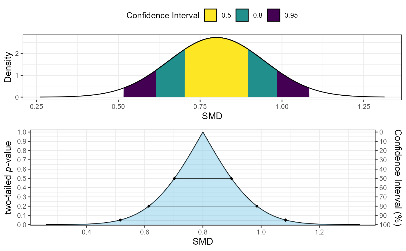
# Example 4: Custom confidence levels
plot_smd(d = 0.8, df = 50, sigma = 0.145, smd_ci = "z",
         levels = c(0.5, 0.8, 0.95))


# Example 5: Using with TOSTER results (requires extracting needed parameters)
# tost_result <- t_TOST(x = group1, y = group2, eqb = 0.5)
# plot_smd(d = tost_result$smd$d,
#          df = tost_result$smd$d_df,
#          sigma = tost_result$smd$d_sigma,
#          smd_ci = "z",
#          smd_label = tost_result$smd$smd_label)

# Example 6: Saving and further customizing the plot
if (FALSE) { # \dontrun{
library(ggplot2)
p <- plot_smd(d = 0.5, df = 40, sigma = 0.164, smd_ci = "z")
p + theme_minimal() +
  labs(title = "Consonance Plot for Cohen's d = 0.5",
       subtitle = "df = 40")
} # }