Joint Confidence Region for Intercept and Slope

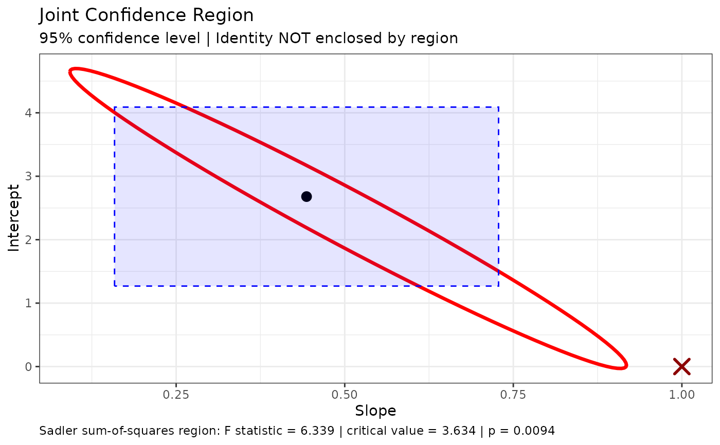
joint_test() tests whether the estimated intercept and slope jointly fall within a confidence region around specified ideal values (typically intercept = 0 and slope = 1 for method comparison studies). plot_joint() draws that region, with the ideal point marked as enclosed or not.

Usage

joint_test(object, ...)

# S3 method for class 'simple_eiv'
joint_test(
  object,
  ideal_intercept = 0,
  ideal_slope = 1,
  conf.level = NULL,
  test_method = c("F", "asymptotic"),
  method = NULL,
  ...
)

plot_joint(x, ...)

# S3 method for class 'simple_eiv'
plot_joint(
  x,
  ideal_intercept = 0,
  ideal_slope = 1,
  conf.level = NULL,
  test_method = c("F", "asymptotic"),
  show_intervals = TRUE,
  n_points = 100,
  method = NULL,
  ...
)

Arguments

object, x

A simple_eiv object from dem_reg() or pb_reg().

...

Additional arguments (currently unused).

ideal_intercept

The hypothesized intercept value (default: 0).

ideal_slope

The hypothesized slope value (default: 1).

conf.level

Confidence level for the region and test. The default, NULL, uses the level the model was fitted with (object$conf.level).

test_method

Reference distribution for the Wald test and ellipse (method = "wald" only). "F" (default) uses F(2, n-2); "asymptotic" uses chi-squared(2), the large-sample approximation. The Sadler test always uses F(2, n-2).

method

Which joint region and test. NULL (default) uses "sadler" for Deming fits and "wald" for Passing-Bablok fits. "sadler" is the sum-of-squares region of Sadler (2010), available for dem_reg() fits only. "wald" is the ellipse from the variance-covariance matrix (the only option for pb_reg()). See Details.

show_intervals

Logical (plot_joint() only). If TRUE (default), also shows the model's marginal confidence intervals as a rectangle. They are shown only when conf.level matches the level the model was fitted with.

n_points

Number of points used to draw the region (plot_joint() only; default 100).

Value

plot_joint() returns a ggplot. joint_test() returns an object of class htest containing:

statistic

For method = "sadler", the F statistic; for method = "wald", the Mahalanobis distance.

parameter

Degrees of freedom. For the F-based tests, df1 and df2; for the asymptotic test, df (always 2).

p.value

The p-value for the test.

conf.int

The confidence level used.

estimate

Named vector of estimated intercept and slope.

null.value

Named vector of hypothesized intercept and slope.

alternative

Description of the alternative hypothesis.

method

Description of the test.

data.name

Name of the input object.

Details

Sadler region (Deming, default)

For a Deming fit with error ratio \(\lambda\) and weights \(w_i\), let $$S(a, b) = \sum_i \frac{w_i (y_i - a - b x_i)^2}{1 + \lambda b^2},$$ the weighted sum of squares that Deming regression minimises (Sadler, 2010, Eq. 11; Draper & Smith). With \(\hat S\) its minimum, the test of \((a_0, b_0)\) is $$F = \frac{(S(a_0, b_0) - \hat S) / 2}{\hat S / (n - 2)}$$ on F(2, n - 2), and the confidence region is the set of \((a, b)\) where \(F\) does not exceed the critical value. No variance-covariance matrix is involved; only the error ratio (not the size of the errors) matters. The region is not an ellipse: for each slope its intercept limits have a closed form, and its slope limits are the roots of a quadratic, so plot_joint() draws it exactly. If the data are too imprecise for the slope to be bounded, the test is still reported but the region is not drawn.

In simulations with normal errors (n = 10 to 100, narrow and wide ranges, error ratios 1 and 4, constant and proportional errors, and replicate data with the error ratio estimated), the Sadler test rejected a true null hypothesis 4.3-5.9% of the time at a nominal 5%. It was at least as powerful as the Wald test at the same size.

The model frame must be stored (dem_reg(model = TRUE), the default). dem_reg(weighted = TRUE) uses fixed weights computed from the data, while Sadler reweighted iteratively; the region uses the fitted model's weights.

Wald ellipse

method = "wald" computes the Mahalanobis distance between the estimated coefficients and the hypothesized values, using the variance-covariance matrix of the estimates, against 2 F(2, n - 2) (or chi-squared(2) with test_method = "asymptotic").

For Deming regression the matrix is the delete-one jackknife. This test is liberal in small samples: in the same simulations it rejected a true null 7.8-9.7% of the time at n = 10, about 7.4% at n = 20 and 6.1% at n = 50 (up to 14% with test_method = "asymptotic"), because the jackknife variance is itself unstable. Prefer the Sadler test for Deming fits.

For Passing-Bablok regression the model must have been fitted with replicates > 0 and se_method = "bootstrap" or "jackknife". Both held 4.3-5.4% in simulations (n = 20 to 100). The Dufey (2020) matrix (se_method = "dufey") is not used for joint tests: it rejected a true null 8-11% of the time.

References

Sadler, W.A. (2010). Joint parameter confidence regions improve the power of parametric regression in method-comparison studies. Accreditation and Quality Assurance, 15, 547-554.

Draper, N.R., & Smith, H. (1966). Applied Regression Analysis. Wiley, New York.

Examples

data("reps")
fit <- dem_reg(y ~ x, data = reps)
joint_test(fit)
#> 
#> 	Joint Confidence Region Test [Sadler sum-of-squares, F-based] (H0:
#> 	intercept = 0, slope = 1)
#> 
#> data:  y ~ x
#> F = 6.3387, df1 = 2, df2 = 16, p-value = 0.009389
#> alternative hypothesis: true intercept and slope are not equal to the null values
#> null values:
#> intercept     slope 
#>         0         1 
#> sample estimates:
#> intercept     slope 
#> 2.6793028 0.4433897 
#> 
plot_joint(fit)


# The Wald ellipse from the jackknife variance-covariance matrix
joint_test(fit, method = "wald")
#> 
#> 	Joint Confidence Region Test [Wald, F-based] (H0: intercept = 0, slope
#> 	= 1)
#> 
#> data:  y ~ x
#> X-squared = 17.172, df1 = 2, df2 = 16, p-value = 0.002929
#> alternative hypothesis: true intercept and slope are not equal to the null values
#> null values:
#> intercept     slope 
#>         0         1 
#> sample estimates:
#> intercept     slope 
#> 2.6793028 0.4433897 
#>