Errors-in-Variables Regression
Aaron R. Caldwell
Last Updated: 2026-03-24
Source:vignettes/Deming.Rmd
Deming.RmdBackground
Error-in-variables (EIV) models are useful tools to account for measurement error in the independent variable. For studies of agreement, this is particularly useful where there are paired measurements of the paired measurements (X & Y) of the same underlying value (e.g., two assays of the same analyte).
Deming regression is one of the simplest forms of of EIV models promoted by W. Edwards Deming1. The first to detail the method were Adcock (1878) followed by Kummell (1879) and Koopmans (1936). The name comes from the popularity of Deming’s book (Deming 1943), and within the field of clinical chemistry, the procedure was simply referred to as “Deming regression” (e.g., Linnet (1990)).
Deming Regression
Simple Deming Regression
We can start by creating some fake data to work with.
library(SimplyAgree)

dat = data.frame(
  x = c(7, 8.3, 10.5, 9, 5.1, 8.2, 10.2, 10.3, 7.1, 5.9),
  y = c(7.9, 8.2, 9.6, 9, 6.5, 7.3, 10.2, 10.6, 6.3, 5.2)
)
Also, we will assume, based on historical data, that the measurement error ratio is equal to 2.
The data can be run through the dem_reg function and the
results printed.
dem1 = dem_reg(y ~ x,
               data = dat,
               error.ratio = 2,
               weighted = FALSE)
dem1
#> Deming Regression with 95% C.I.
#>
#> Call:
#> dem_reg(formula = y ~ x, data = dat, weighted = FALSE, error.ratio = 2,
#>     conf.level = 0.95)
#>
#> Coefficients:
#> (Intercept)           x
#>      0.1285      0.9745
The resulting regression line can then be plotted.
plot(dem1, interval = "confidence")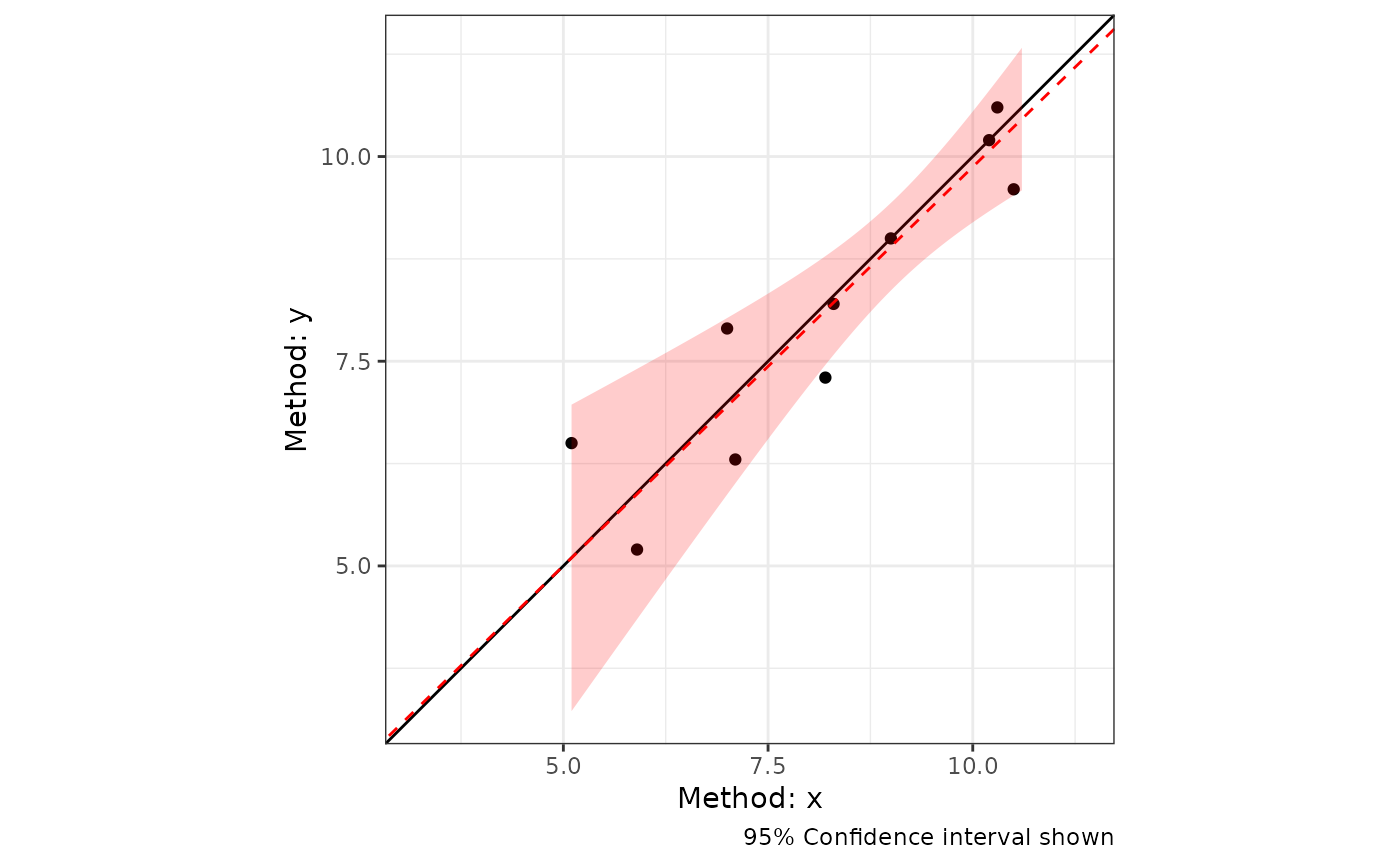
Model Diagnostics
The assumptions of the Deming regression model, primarily normality
and homogeneity of variance, can then be checked with the
check method for Deming regression results. Both plots
appear to be fine with regards to the assumptions.
check(dem1)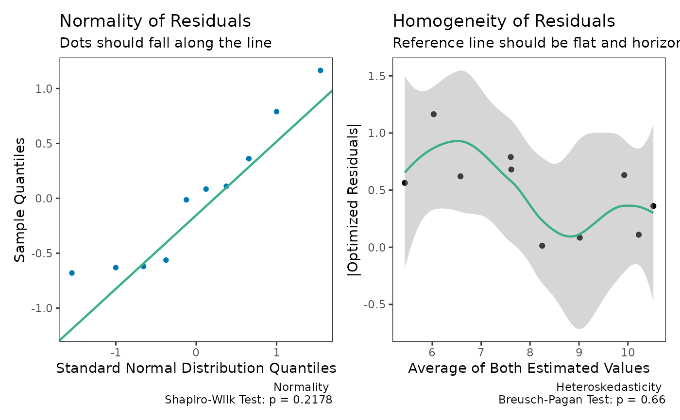
Fitted Values and Residuals
After fitting a Deming regression model, you can extract the
estimated true values and residuals. The fitted() function
returns the estimated true Y values, accounting for measurement error.
The residuals() function returns the optimized residuals by
default, which correspond to the perpendicular distances from each point
to the regression line.
Weighted Deming Regression
For this example, I will rely upon the “ferritin” data from the
deming R package.
library(deming)
data('ferritin')

head(ferritin)
#>   id period old.lot new.lot
#> 1  1      1       1       1
#> 2  2      1       3       3
#> 3  3      1      10       9
#> 4  4      1      13      11
#> 5  5      1      13      12
#> 6  6      1      15      13
Let me demonstrate the problem with using simple Deming regression when the weights are helpful. When we look at the two plots below, we can see there is severe problem with using the “un-weighted” model.
dem2 = dem_reg(
  old.lot ~ new.lot,
  data = ferritin,
  weighted = FALSE
)
summary(dem2)
#> Deming Regression with 95% C.I.
#>
#> Call:
#> dem_reg(formula = old.lot ~ new.lot, data = ferritin, weighted = FALSE,
#>     conf.level = 0.95)
#>
#> Coefficients:
#>             coef      bias      se  df lower.ci upper.ci      t p.value
#> Intercept 5.2157 -0.235818 2.18603 160   0.8985    9.533  2.386 0.01821
#> Slope     0.9637  0.002597 0.02505 160   0.9143    1.013 -1.448 0.14949
#>
#> 160 degrees of freedom
#> Error variance ratio (lambda): 1.0000

plot(dem2)
check(dem2)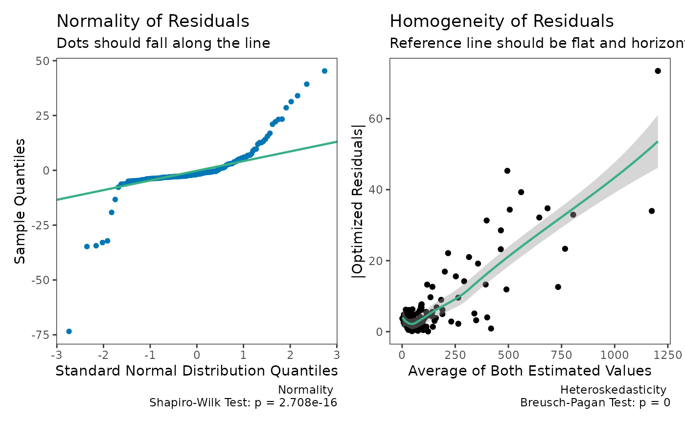
Now, let us see what happens when weighted is set to
TRUE.
dem3 = dem_reg(
  old.lot ~ new.lot,
  data = ferritin,
  weighted = TRUE
)
summary(dem3)
#> Weighted Deming Regression with 95% C.I.
#>
#> Call:
#> dem_reg(formula = old.lot ~ new.lot, data = ferritin, weighted = TRUE,
#>     conf.level = 0.95)
#>
#> Coefficients:
#>               coef       bias       se  df lower.ci upper.ci       t   p.value
#> Intercept -0.02616  0.0065148 0.033219 160 -0.09176  0.03945 -0.7874 4.322e-01
#> Slope      1.03052 -0.0001929 0.006262 160  1.01815  1.04288  4.8729 2.626e-06
#>
#> 160 degrees of freedom
#> Error variance ratio (lambda): 1.0000

plot(dem3)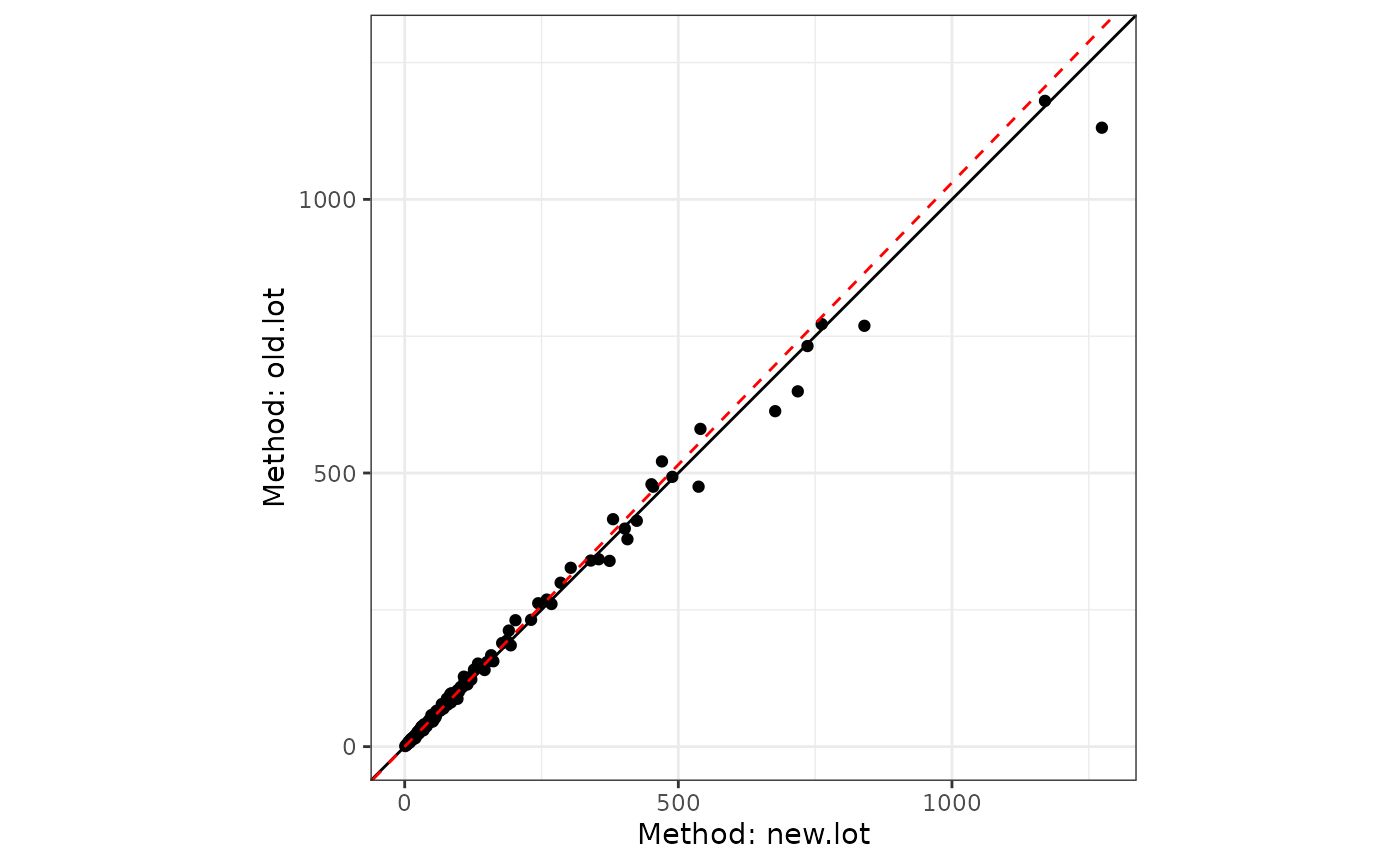
check(dem3)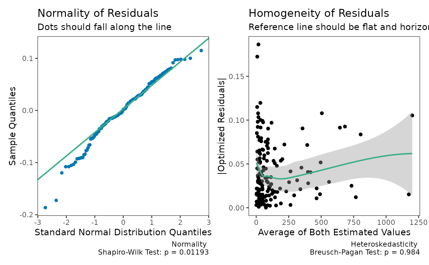
The weighted model provides a better fit.
Passing-Bablok Regression
Passing-Bablok regression is a robust, nonparametric alternative to Deming regression for method comparison studies (Passing and Bablok 1983). Unlike Deming regression, it makes no assumptions about the distribution of the measurement errors. The method estimates the slope as the shifted median of all pairwise slopes between data points, which makes it resistant to outliers.
When to Use Passing-Bablok
Passing-Bablok regression is particularly useful when:
- Both X and Y are measured with error
- You want a robust method not sensitive to outliers
- The relationship is assumed to be linear
- X and Y are highly positively correlated
Basic Usage
The pb_reg() function implements three variants of
Passing-Bablok regression:
- “scissors” (default): Most robust, scale-invariant method from Bablok et al. (1988)
- “symmetric”: Original method from Passing and Bablok (1983)
- “invariant”: Scale-invariant method from Passing and Bablok (1984)
# Create example data
pb_data <- data.frame(
  method1 = c(69.3, 27.1, 61.3, 50.8, 34.4, 92.3, 57.5, 45.5, 33.3, 60.9,
              56.3, 49.9, 89.7, 28.9, 96.3, 76.6, 83.2, 79.4, 51.7, 32.5,
              99.1, 14.2, 84.1, 48.8, 61.5, 84.9, 93.2, 73.8, 62.1, 98.6),
  method2 = c(69.1, 26.7, 61.4, 51.2, 34.7, 88.5, 57.9, 45.1, 33.4, 60.8,
              66.5, 48.2, 88.3, 29.3, 96.4, 77.1, 82.7, 78.9, 51.6, 28.8,
              98.4, 12.7, 83.6, 47.3, 61.2, 84.6, 92.1, 73.4, 61.9, 98.6)
)

# Fit Passing-Bablok regression
pb1 <- pb_reg(method2 ~ method1, data = pb_data)
#> Warning in pb_reg(method2 ~ method1, data = pb_data): Bootstrap confidence
#> intervals are recommended for 'invariant' and 'scissors' methods. Consider
#> setting replicates > 0.
pb1
#> Passing-Bablok (scissors) with 95% C.I.
#>
#> Call:
#> pb_reg(formula = method2 ~ method1, data = pb_data)
#>
#> Coefficients:
#> (Intercept)     method1
#>     0.09622     0.99440
#>
#> Kendall's Tau (H0: tau <= 0):
#>   tau:       0.9632
#>   p-value:   0.0000
#>
#> CUSUM Linearity Test:
#>   Test stat: 1.0000
#>   p-value:   0.1844
Summary and Plots
The summary provides details about the regression coefficients and diagnostic tests:
summary(pb1)
#> Passing-Bablok (scissors) with 95% C.I.
#>
#> Call:
#> pb_reg(formula = method2 ~ method1, data = pb_data)
#>
#> Coefficients:
#>        term    coef       se lower.ci upper.ci df null_value reject_h0
#> 1 Intercept 0.09622 0.390603  -0.7206   0.8105 28          0     FALSE
#> 2   method1 0.99440 0.005918   0.9840   1.0072 28          1     FALSE
#>
#> 28 degrees of freedom
#> Error variance ratio (lambda): 1.0000
The plot() method displays the regression line with
data:
plot(pb1)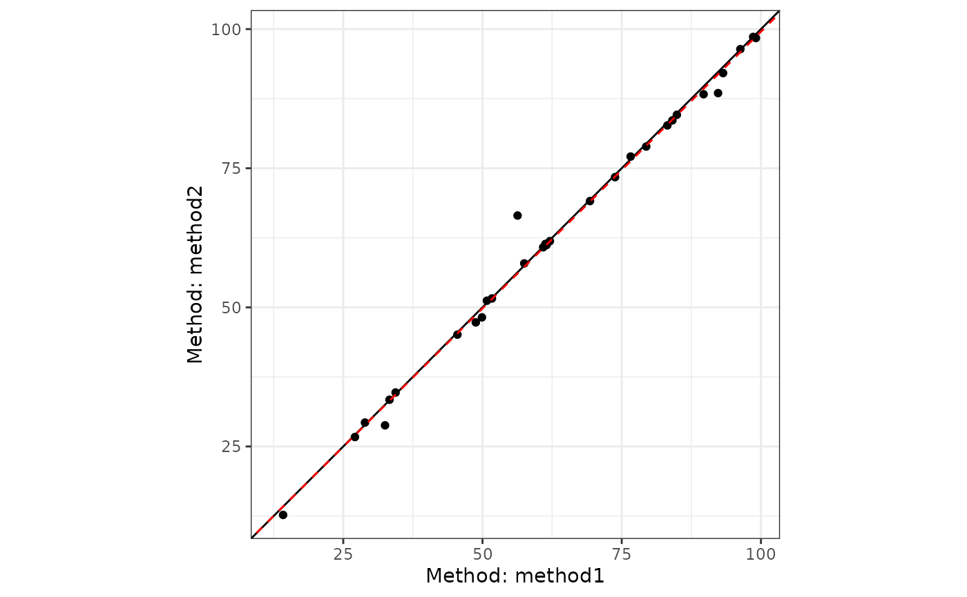
Model Diagnostics
The check() method provides diagnostic plots specific to
Passing-Bablok regression, including the CUSUM linearity test and
Kendall’s tau correlation:
check(pb1)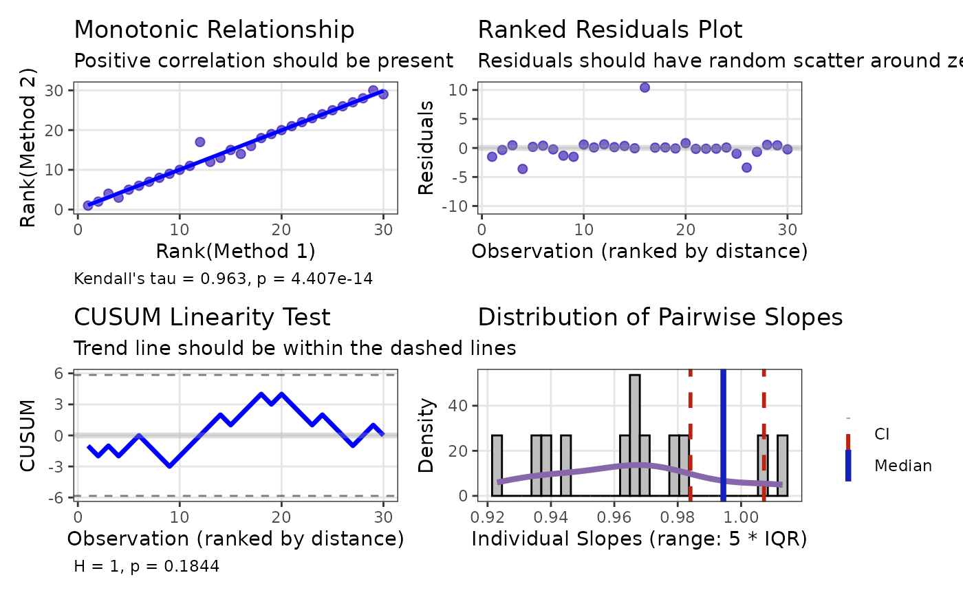
Bootstrap Confidence Intervals
For more robust inference, especially with the “invariant” or “scissors” methods, bootstrap confidence intervals are recommended:
pb2 <- pb_reg(method2 ~ method1,
              data = pb_data,
              replicates = 999)
summary(pb2)
#> Passing-Bablok (scissors) with 95% C.I.
#>
#> Call:
#> pb_reg(formula = method2 ~ method1, data = pb_data, replicates = 999)
#>
#> Coefficients:
#>        term    coef       se lower.ci upper.ci df null_value reject_h0
#> 1 Intercept 0.09622 0.088205 -0.09182   0.2539 28          0     FALSE
#> 2   method1 0.99440 0.001291  0.99198   0.9970 28          1      TRUE
#>
#> 28 degrees of freedom
#> Error variance ratio (lambda): 1.0000
#>
#>
#> Bootstrap CIs based on 999 resamples
Joint Confidence Regions
A theoretically valid, but still experimental, enhancement to the
dem_reg and pb_reg functions is the addition
of joint confidence regions for the slope and intercept
parameters. Traditional confidence intervals treat each parameter
separately, but in regression analysis, these parameters are
correlated.
Joint confidence regions account for this correlation by creating an elliptical region in the (intercept, slope) parameter space. This approach, promoted by Sadler (2010), provides several advantages:
- Higher Statistical Power: The ellipse typically requires 20-50% fewer samples than traditional confidence intervals to detect the same bias
- Accounts for Parameter Correlation: When the measurement range is narrow, slope and intercept are highly negatively correlated
- More Appropriate Test: Testing against a point (e.g., slope=1, intercept=0) is naturally done with a region, not separate intervals
The power advantage is most pronounced when the ratio of maximum to minimum X values is small (< 10:1), which is common in clinical method comparisons.
Visualizing the Joint Confidence Region
The plot_joint() function allows visualization of the
confidence region in parameter space:
plot_joint(dem1,
           ideal_slope = 1,
           ideal_intercept = 0,
           show_intervals = TRUE)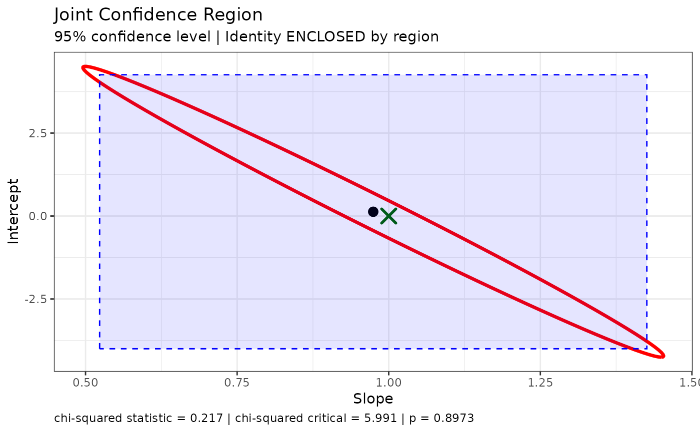
This plot shows:
- The red ellipse: Joint confidence region
- The blue rectangle: Traditional confidence intervals
- The black dot: Estimated (intercept, slope)
- The green/red X: Ideal point (whether enclosed or not)
Notice how the ellipse is smaller than the rectangle, especially in the directions that matter for detecting bias.
For Passing-Bablok regression, bootstrap resampling must be used to obtain the variance-covariance matrix needed for the joint confidence region:
plot_joint(pb2)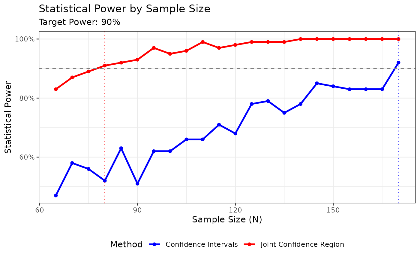
Joint Hypothesis Test
The joint_test() function provides a formal hypothesis
test for whether the identity line (slope = 1, intercept = 0) falls
within the joint confidence region:
joint_test(dem1)
#>
#>  Joint Confidence Region Test (H0: intercept = 0, slope = 1)
#>
#> data:  y ~ x
#> X-squared = 0.21666, df = 2, p-value = 0.8973
#> alternative hypothesis: true intercept and slope are not equal to the null values
#> null values:
#> intercept     slope
#>         0         1
#> sample estimates:
#> intercept     slope
#> 0.1284751 0.9744516
This returns an htest object with the Mahalanobis
distance (chi-squared statistic) and p-value. The test can also be
applied to Passing-Bablok models fitted with bootstrap:
joint_test(pb2)
#>
#>  Joint Confidence Region Test (H0: intercept = 0, slope = 1)
#>
#> data:  method2 ~ method1
#> X-squared = 905.61, df = 2, p-value < 2.2e-16
#> alternative hypothesis: true intercept and slope are not equal to the null values
#> null values:
#> intercept     slope
#>         0         1
#> sample estimates:
#>  intercept      slope
#> 0.09621849 0.99439776
Theoretical Details
Deming Calculative Approach
Deming regression assumes paired measures (\(x_i, \space y_i\)) are each measured with error.
\[ x_i = X_i + \epsilon_i \]
\[ y_i = Y_i + \delta_i \]
We can then measure the relationship between the two variables with the following model.
\[ \hat Y_i = \beta_0 + \beta_1 \cdot \hat X_i \]
Traditionally there are 2 null hypotheses.
First, the intercept is equal to zero:
\[ H_0: \beta_0 = 0 \space vs. \space H_1: \beta_0 \ne 0 \]
Second, that the slope is equal to one:
\[ H_0: \beta_1 = 1 \space vs. \space H_1: \beta_0 \ne 1 \]
Joint Confidence Region Calculative Approach
The joint \((1-\alpha) \times 100\%\) confidence region for \((\beta_0, \beta_1)\) is defined as:
\[ (\hat{\beta} - \beta_0)^T V^{-1} (\hat{\beta} - \beta_0) \leq \chi^2_{2,\alpha} \]
Where:
- \(\hat{\beta}\) = estimated parameters \((\hat{\beta}_0, \hat{\beta}_1)\)
- \(\beta_0\) = hypothesized parameters (e.g., \((0, 1)\) for identity)
- \(V\) = variance-covariance matrix
- \(\chi^2_{2,\alpha}\) = chi-square critical value with 2 degrees of freedom
This forms an ellipse in parameter space that accounts for the correlation between slope and intercept.
Measurement Error
A Deming regression model also assumes the measurement error (\(\sigma^2\)) ratio is constant.
\[ \lambda = \frac{\sigma^2_\epsilon}{\sigma^2_\delta} \]
In SimplyAgree, the error ratio can be set with the
error.ratio argument. It defaults to 1, but can be changed
by the user. If replicate measures are taken, then the user can use the
id argument to indicate which measures belong to which
subject/participant. The measurement error, and the error ratio, will
then be estimated from the data itself.
If the data was not measured in replicate then the error ratio (\(\lambda\)) can be estimated from the coefficient of variation (if that data is available) and the mean of x and y (\(\bar x, \space \bar y\)).
\[ \lambda = \frac{(CV_y \cdot \bar y)^2}{(CV_x \cdot \bar x)^2} \]
Weights
In some cases the variance of X and Y may increase proportional to
the true value of the measure. In these cases, it may be prudent to use
“weighted” Deming regression models. The weights used in
SimplyAgree are the same as those suggested by Linnet (1993).
\[ \hat w_i = \frac{1}{ [ \frac{x_i + \lambda \cdot y_i}{1 + \lambda}]^2} \]
Weights can also be provided through the weights
argument. If weighted Deming regression is not selected
(weighted = FALSE), the weights for each observation is
equal to 1.
The estimated mean of X and Y are then estimated as the following.
\[ \bar x_w = \frac{\Sigma^{N}_{i=1} \hat w_i \cdot x_i}{\Sigma^{N}_{i=1} \hat w_i} \]
\[ \bar y_w = \frac{\Sigma^{N}_{i=1} \hat w_i \cdot y_i}{\Sigma^{N}_{i=1} \hat w_i} \]
Estimating the Slope and Intercept
First, there are 3 components (\(v_x, \space v_y, \space cov_{xy}\))
\[ v_x = \Sigma_{i=1}^N \space \hat w_i \cdot (x_i- \bar x_w)^2 \] \[ v_y = \Sigma_{i=1}^N \space \hat w_i \cdot (y_i- \bar y_w)^2 \] \[ cov_{xy} = \Sigma_{i=1}^N \space \hat w_i \cdot (x_i- \bar x_w) \cdot (y_i- \bar y_w) \]
The slope (\(b_1\)) can then be estimated with the following equation.
\[ b_1 = \frac{(\lambda \cdot v_y - v_x) + \sqrt{(v_x-\lambda \cdot v_y)^2 + 4 \cdot \lambda \cdot cov_{xy}^2}}{2 \cdot \lambda \cdot cov_{xy}} \]
The intercept (\(b_0\)) can then be estimated with the following equation.
\[ b_0 = \bar y_w - b_1 \cdot \bar x_w \]
The standard errors of b1 and b0 are both estimated using a jackknife method (detailed by Linnet (1990)).