library(SimplyAgree)
#library(tidyverse)
library(dplyr)
library(tidyr)
library(ggplot2)
library(magrittr)
data("temps")
df_temps = temps
Re-analysis of a Previous Study of Agreement
In the study by Ravanelli and Jay (2020), they attempted to estimate the effect of varying the time of day (AM or PM) on the measurement of thermoregulatory variables (e.g., rectal and esophageal temperature). In total, participants completed 6 separate trials wherein these variables were measured. While this is a robust study of these variables the analyses focused on ANOVAs and t-tests to determine whether or not the time-of-day (AM or PM). This poses a problem because 1) they were trying to test for equivalence and 2) this is a study of agreement not differences (See Lin (1989)). Due to the latter point, the use of t-test or ANOVAs (F-tests) is rather inappropriate since they provide an answer to different, albeit related, question.
Instead, the authors could test their hypotheses by using tools that
estimate the absolute agreement between the AM and PM sessions
within each condition. This is rather complicated because we have
multiple measurement within each participant. However, with the tools
included in SimplyAgree1 I believe we can get closer to the right
answer.
In order to understand the underlying processes of these functions
and procedures I highly recommend reading the statistical literature
that documents methods within these functions. For the
cccrm package please see the work by Josep L. Carrasco and Jover (2003), Josep L. Carrasco, King, and Chinchilli (2009),
and Josep L. Carrasco et al. (2013). The
tolerance_limit function was inspired by the work of Francq, Berger, and Boachie (2020) which
documented how to implement tolerance limits to measure agreement.
Concordance
An easy approach to measuring agreement between 2 conditions or
measurement tools is through the concordance correlation coefficient
(CCC). The CCC essentially provides a single coefficient (values between
0 and 1) that provides an estimate to how closely one measurement is to
another. It is a type of intraclass correlation coefficient that takes
into account the mean difference between two measurements. In other
words, if we were to draw a line of identity on a graph and plot two
measurements (X & Y), the closer those points are to the line of
identity the higher the CCC (and vice versa). Please see the
cccrm package for more details.
qplot(1,1) + geom_abline(intercept = 0, slope = 1)
#> Warning: `qplot()` was deprecated in ggplot2 3.4.0.
#> This warning is displayed once per session.
#> Call `lifecycle::last_lifecycle_warnings()` to see where this warning was
#> generated.
Example of the Line of Identity
In the following sections, let us see how well esophageal and rectal temperature are in agreement after exercising in the heat for 1 hour at differing conditions.
Rectal Temperature
We can visualize the concordance between the two different types of measurements and the respective time-of-day and conditions. From the plot we can see there is clear bias in the raw post exercise values (higher in the PM), but even when “correcting for baseline differences” by calculating the differences scores we can see a higher degree of disagreement between the two conditions.
#> Warning: Using `size` aesthetic for lines was deprecated in ggplot2 3.4.0.
#> ℹ Please use `linewidth` instead.
#> This warning is displayed once per session.
#> Call `lifecycle::last_lifecycle_warnings()` to see where this warning was
#> generated.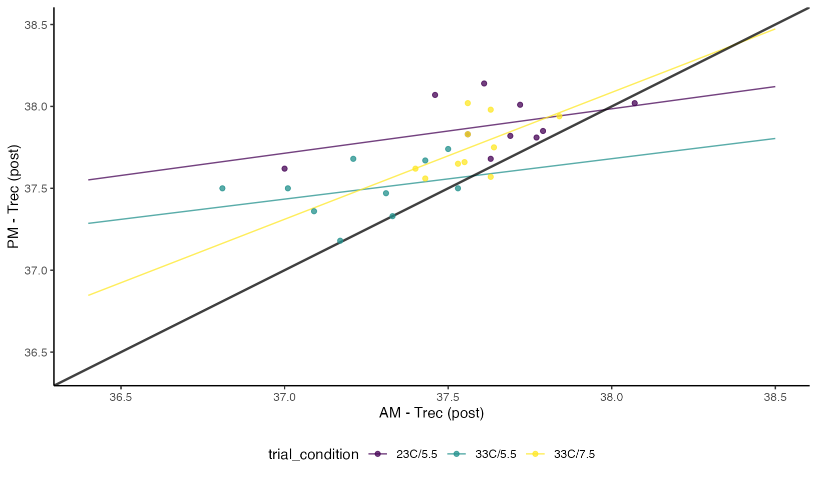
Concordance Plots of Rectal Temperature
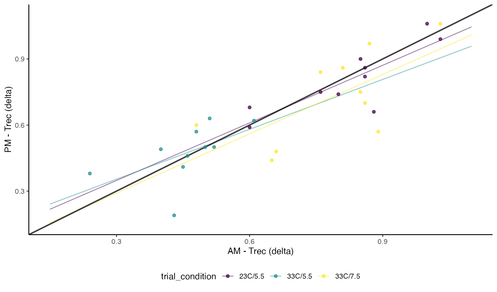
Concordance Plots of Rectal Temperature
Esophageal Temperature
#> Warning: Removed 3 rows containing missing values or values outside the scale range
#> (`geom_line()`).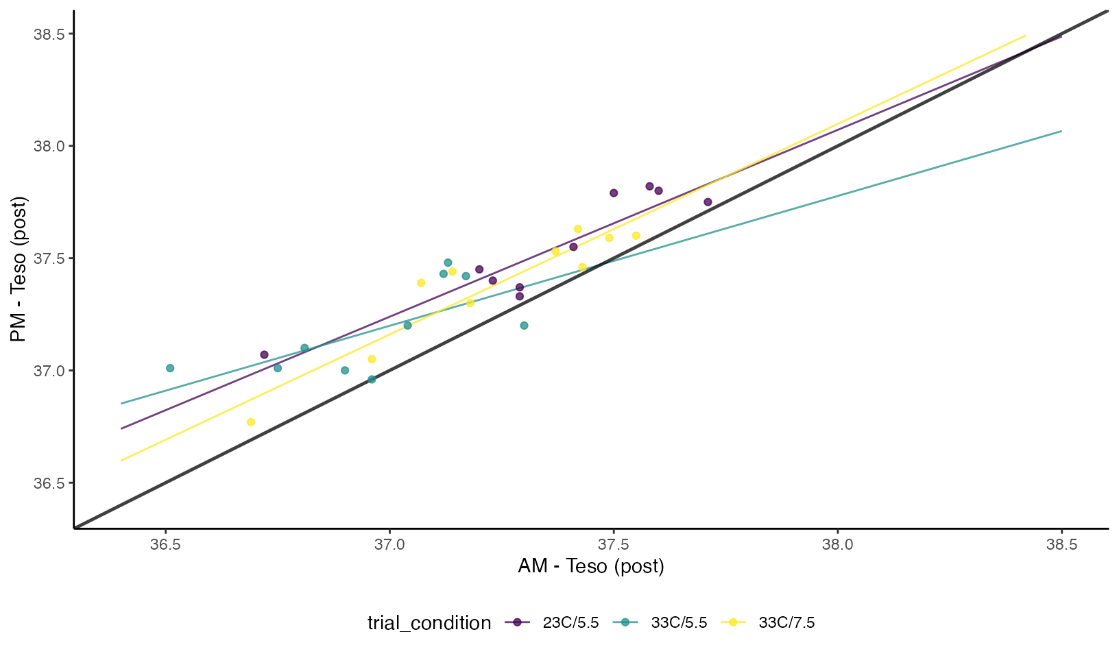
Concordance Plots of Esophageal Temperature
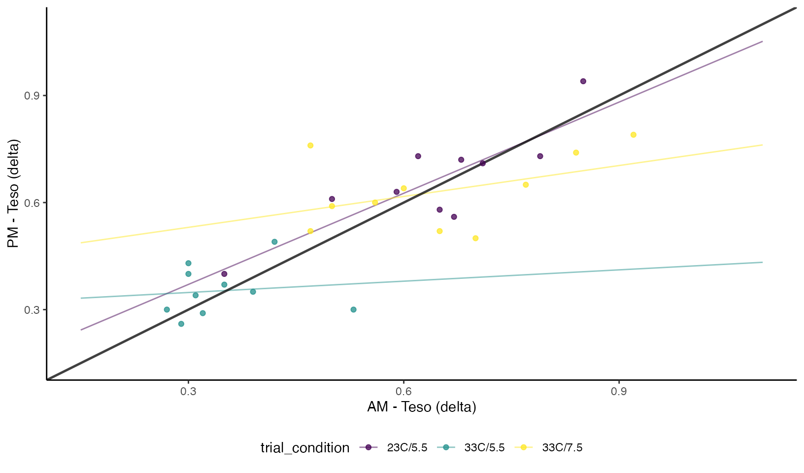
Concordance Plots of Esophageal Temperature
Tolerance Limits to Assess Agreement
The tolerance_limit function can be used to calculate
the “tolerance limits”. Typically a 95% prediction interval is
calculated which provides the predicted difference between two measuring
systems for 95% of future measurements pairs. However, we have to
account for sampling error so we also need to estimate the confidence in
the prediction intervals, and therefore we calculate the tolerance
limits. So, when we have 95% tolerance limits for a 95% prediction
interval, we can conclude that there is only a 5% probability
(1-tolerance) that our tolerance limits do not contain the true
prediction interval/limit.
Rectal Temperature
So we will calculate the tolerance using the loa_lme
function. We will need to identify the columns with the right
information using the diff, avg,
condition, and id arguments. We then select
the right data set using the data argument. Lastly, we
specify the specifics of the conditions for how the limits are
calculated. For this specific analysis I decided to calculate 95%
prediction intervals with 95% tolerance limits, and I will use
percentile bootstrap confidence intervals.
# note: more accurate tolerance limits are given by tol_method = "perc"
rec.post_tol = tolerance_limit(
  data = df_rec.post,
  x = "PM",
  y = "AM",
  id = "id",
  condition = "trial_condition"
)
When we print a table of the tolerance limits, at least for Trec post exercise, are providing the same conclusion (poor agreement).
print(rec.post_tol)
#> Agreement between Measures (Difference: x-y)
#> 95% Prediction Interval with 95% Tolerance Limits
#>
#>  Condition  Bias          Bias CI Prediction Interval  Tolerance Limits
#>    23C/5.5 0.255 [0.0803, 0.4297]   [-0.3245, 0.8345] [-0.5248, 1.0348]
#>    33C/5.5 0.254 [0.0964, 0.4116]   [-0.3144, 0.8224] [-0.4978, 1.0058]
#>    33C/7.5 0.181   [0.021, 0.341]   [-0.7101, 1.0721] [-1.4732, 1.8352]
Furthermore, we can visualize the results with a Bland-Altman style
plot of the tolerance. Notice, despite the tighter cluster in the 3rd
condition, the prediction/tolerance limits are wider. This is a curious
result, but if we inspect the results further
(rec.post_tol$emmeans) we can see the degrees of freedom
for this condition are horribly low.
plot(rec.post_tol)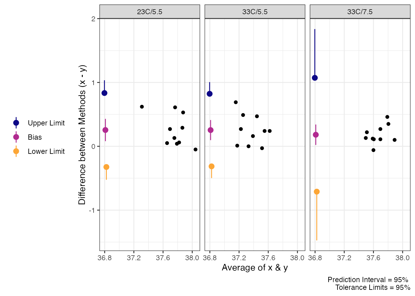
Tolerance Limits for Trec Post Exercise
Now, when we look at the Delta values for Trec we find that there is much closer agreement (maybe even acceptable agreement) when we look at tolerance limits. However, we cannot say that the average difference would be less than 0.25 which may not be acceptable for some researchers.
rec.delta_tol = tolerance_limit(
  x = "PM",
  y = "AM",
  condition = "trial_condition",
  id = "id",
  data = df_rec.delta
)

rec.delta_tol
#> Agreement between Measures (Difference: x-y)
#> 95% Prediction Interval with 95% Tolerance Limits
#>
#>  Condition   Bias           Bias CI Prediction Interval  Tolerance Limits
#>    23C/5.5 -0.019   [-0.084, 0.046]   [-0.2345, 0.1965] [-0.3466, 0.3086]
#>    33C/5.5  0.015 [-0.0625, 0.0925]   [-0.1874, 0.2174] [-0.2646, 0.2946]
#>    33C/7.5 -0.059 [-0.1635, 0.0455]   [-0.2723, 0.1543] [-0.3517, 0.2337]
# Plot Maximal Allowable Difference with delta argument
plot(rec.delta_tol,
     delta = .25)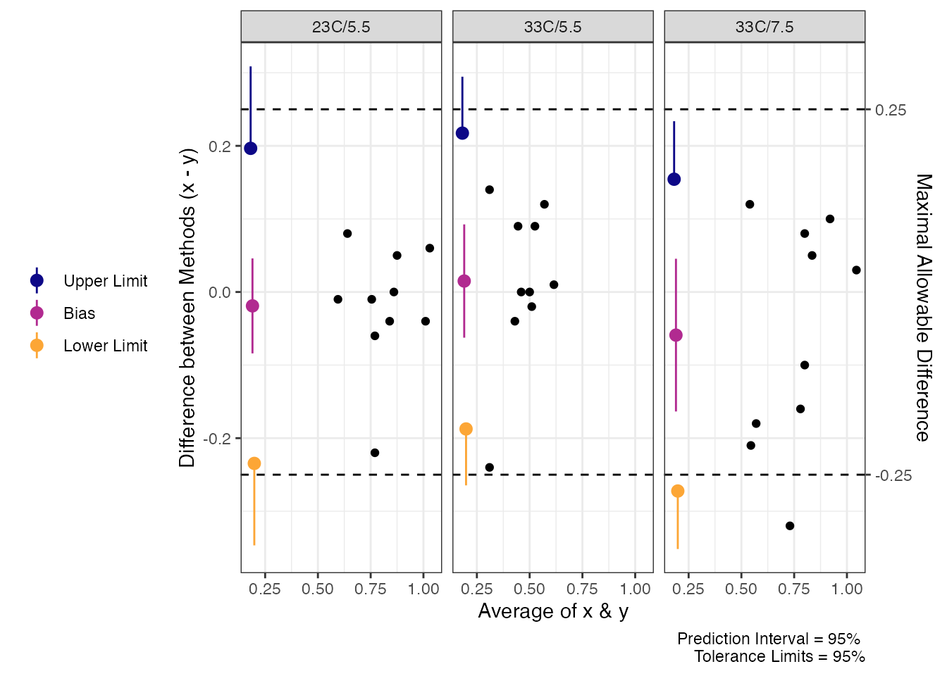
Tolerance Limits for Delta Trec
Esophageal Temperature
We can repeat the process for esophageal temperature. Overall, the results are fairly similar, and while there is better agreement on the delta (change scores), it is still fairly difficult to determine that there is “good” agreement between the AM and PM measurements.
eso.post_tol = tolerance_limit(
  x = "AM",
  y = "PM",
  condition = "trial_condition",
  id = "id",
  data = df_eso.post
)

eso.delta_tol = tolerance_limit(
  x = "AM",
  y = "PM",
  condition = "trial_condition",
  id = "id",
  data = df_eso.delta
)
eso.post_tol
#> Agreement between Measures (Difference: x-y)
#> 95% Prediction Interval with 95% Tolerance Limits
#>
#>  Condition   Bias            Bias CI Prediction Interval  Tolerance Limits
#>    23C/5.5 -0.180 [-0.2564, -0.1036]   [-0.4332, 0.0732]   [-0.556, 0.196]
#>    33C/5.5 -0.212   [-0.329, -0.095]   [-0.4603, 0.0363] [-0.5414, 0.1174]
#>    33C/7.5 -0.146    [-0.23, -0.062]   [-0.4159, 0.1239] [-0.5676, 0.2756]
plot(eso.post_tol)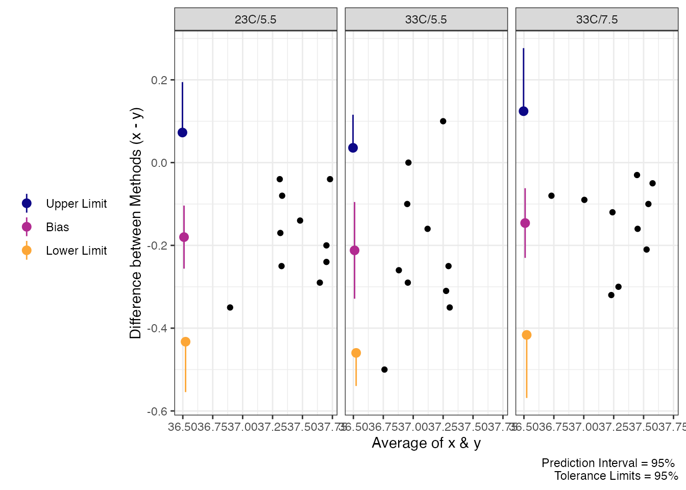
Limits of Agreement for Teso Post Exercise
eso.delta_tol
#> Agreement between Measures (Difference: x-y)
#> 95% Prediction Interval with 95% Tolerance Limits
#>
#>  Condition   Bias           Bias CI Prediction Interval  Tolerance Limits
#>    23C/5.5 -0.020 [-0.0746, 0.0346]   [-0.2012, 0.1612] [-0.2709, 0.2309]
#>    33C/5.5 -0.005 [-0.0721, 0.0621]   [-0.1858, 0.1758] [-0.2458, 0.2358]
#>    33C/7.5  0.017 [-0.0849, 0.1189]   [-0.1826, 0.2166] [-0.2571, 0.2911]
plot(eso.delta_tol,
     delta = .25)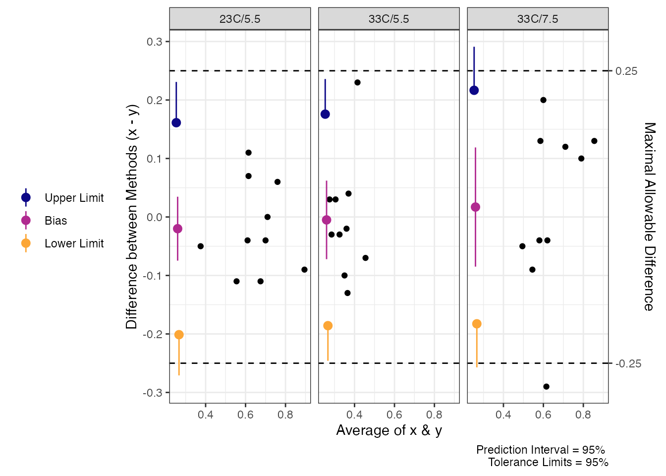
Limits of Agreement for Delta Teso
