Methods for ccc_htest objects

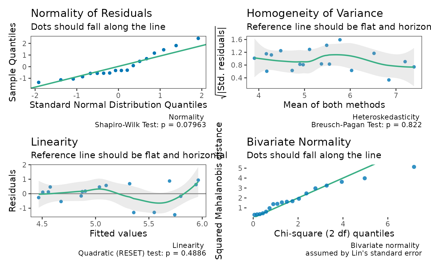
Methods for objects returned by ccc_test(). They print as standard "htest" objects; summary() describes the result in words, plot() shows the agreement between the two methods, and check() gives diagnostics.

Usage

# S3 method for class 'ccc_htest'
summary(object, style = c("auto", "hypothesis", "estimation"), ...)

# S3 method for class 'ccc_htest'
plot(x, type = c("identity", "ba"), ...)

# S3 method for class 'ccc_htest'
check(x, ...)

Arguments

style

How summary() words the result: "auto" (default), "hypothesis", or "estimation", as for icc_test() results (see reli_htest-methods).

...

Not used.

x, object

An object of class ccc_htest.

type

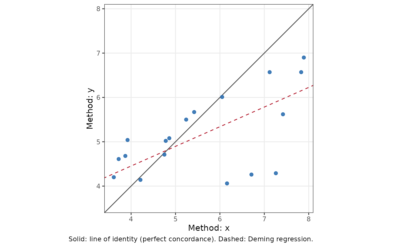
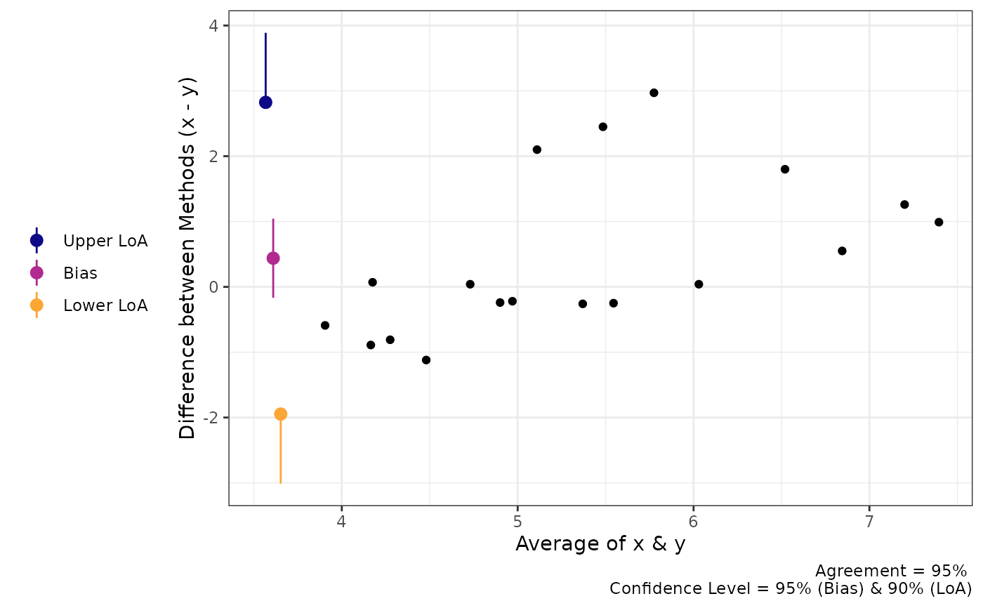
For plot(): "identity" (default), the measurements of y against x with the line of identity (perfect concordance) and a Deming regression line, coloured by subject for replicate or nested data; or "ba", the Bland-Altman plot of the differences against the means (from agreement_limit() with the same data type).

Value

summary

An object of class summary.ccc_htest (which prints like summary.reli_htest): the description in text, the style used, the S-value (s.value, when there is a p-value), and the parts used to build it.

plot

A ggplot2 plot (see type).

check

Diagnostic plots combined with patchwork.

Details

summary() describes the estimate and its interval, what was estimated, the design, and how the inference was done, in the hypothesis or estimation style described in reli_htest-methods. For simple paired data it also reports Lin's decomposition of the CCC into precision (the Pearson correlation, r) and accuracy (the bias correction factor, C_b): CCC = r x C_b. A low CCC can come from either.

check() shows the normality and heteroskedasticity of the differences (as for agreement_limit() with the same data), and the linearity of the relationship between the methods: the residuals of y regressed on x against the fitted values, with a test of a quadratic term (Ramsey's RESET test). The CCC, through its precision component, summarises a linear relationship. Proportional bias is not shown: a slope different from 1 between the methods lowers the bias correction factor C_b, so it is part of what the CCC measures rather than a violation of its assumptions. For simple paired data check() also shows a Q-Q plot of the squared Mahalanobis distances of the pairs against a chi-square distribution with 2 degrees of freedom: Lin's standard error assumes the two measurements are bivariate normal, and points far above the line suggest they are not. For replicate or nested data the linearity test uses all pairs, which are correlated within subjects, so its p-value is approximate; the jackknife standard error makes few distributional assumptions, so these panels mainly help interpret the CCC.

References

Lin, L. I. (1989). A concordance correlation coefficient to evaluate reproducibility. Biometrics, 45(1), 255-268. doi:10.2307/2532051

Carrasco, J. L., & Jover, L. (2003). Estimating the generalized concordance correlation coefficient through variance components. Biometrics, 59(4), 849-858. doi:10.1111/j.0006-341x.2003.00099.x

Ramsey, J. B. (1969). Tests for specification errors in classical linear least-squares regression analysis. Journal of the Royal Statistical Society: Series B, 31(2), 350-371. doi:10.1111/j.2517-6161.1969.tb00796.x

Examples

data("reps")
res <- ccc_test(x = "x", y = "y", data = reps)
summary(res)
#> The estimated CCC was 0.479 (95% compatibility interval [0.128,
#> 0.724]). Values in this interval are the most compatible with the data,
#> given the model and its assumptions. The estimate is Lin's concordance
#> correlation coefficient between x and y: how closely the pairs fall on
#> the line of identity. It combines precision (Pearson r = 0.577) and
#> accuracy (bias correction factor C_b = 0.831), CCC = r x C_b. The data
#> had 18 complete pairs. The interval uses Fisher's z transformation with
#> Lin's (1989) delta-method standard error, which assumes the two
#> measurements are bivariate normal.
plot(res)

plot(res, type = "ba")

check(res)