Methods for reli_htest objects — reli_htest-methods • SimplyAgree

Methods for objects returned by icc_test(), reli_err_test(), reli_facet_test() and mdc_test(). They print as standard "htest" objects; summary() describes the result in words, plot() shows the data, and check() gives model diagnostics.

Usage

# S3 method for class 'reli_htest'
summary(object, style = c("auto", "hypothesis", "estimation"), ...)

# S3 method for class 'summary.reli_htest'
print(x, ...)

# S3 method for class 'reli_htest'
plot(x, type = c("profile", "subjects", "items", "pairs", "components"), ...)

# S3 method for class 'reli_htest'
check(x, ...)

Arguments

style: How summary() words the result: "auto" (default), "hypothesis", or "estimation". "auto" uses "hypothesis" when the result has a p-value (a null.value was given) and "estimation" otherwise. See Details.
...: Not used.
x, object: An object of class reli_htest.
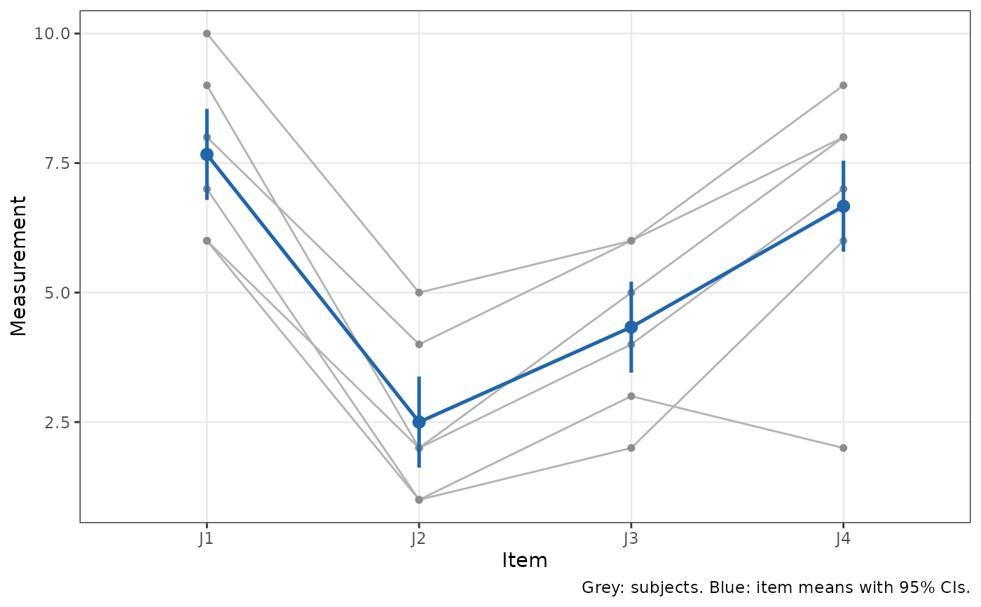
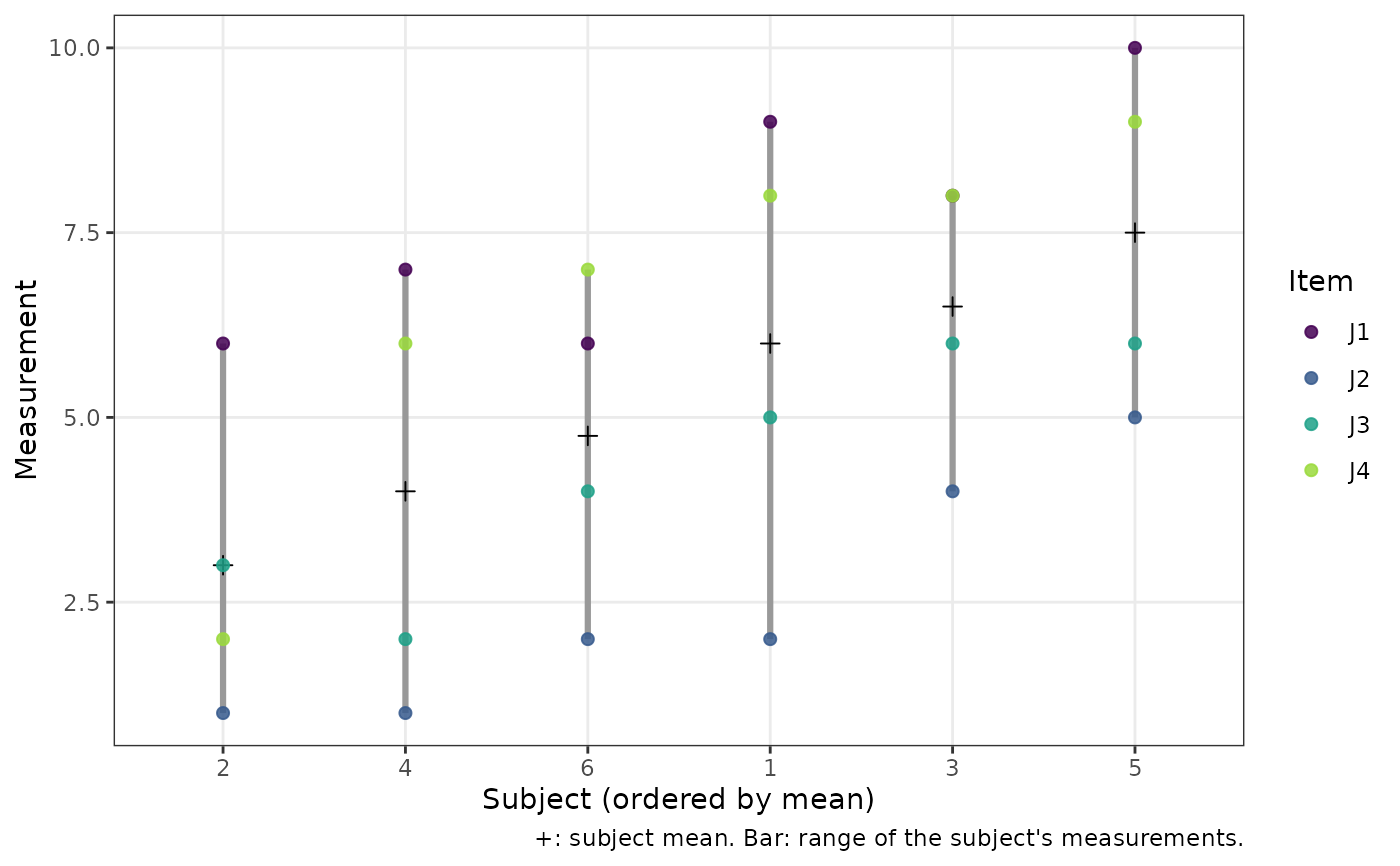
type: For plot(), the plot to draw: "profile" (default), each subject's measurements across the items in grey with the item means and their 95% confidence intervals (adjusted for subjects when measurements are missing); "subjects", the subjects ordered by their mean, with each subject's measurements, coloured by item, and their range, which compares the spread between subjects with the scatter within subjects (what the ICC summarises); "items", the deviation of each measurement from its subject's mean, by item, which shows systematic differences between items (error for an agreement ICC, but not for a consistency ICC); "pairs", each pair of items plotted against each other with the line of identity; or, for reli_facet_test() results, "components", the share of each variance component. For reli_facet_test() results the profile, items and pairs plots use the subject-by-item cell means.

Value

summary: An object of class summary.reli_htest: a list with the description in text, the style used, the S-value (s.value, when there is a p-value) and the parts used to build it. It prints as a paragraph.
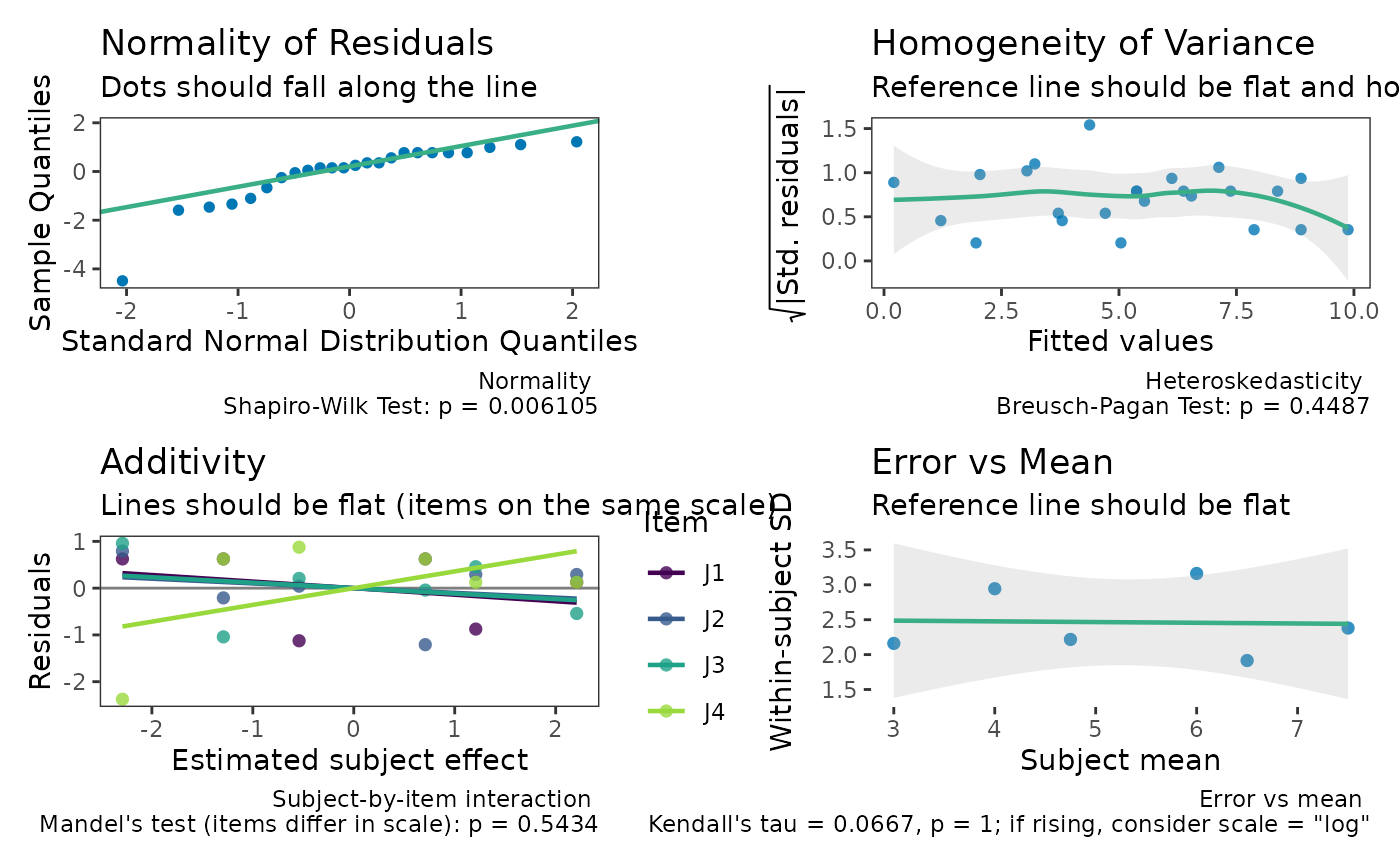
plot: A ggplot2 plot (see type).
check: Diagnostic plots combined with patchwork: normality and heteroskedasticity of the model residuals; for two-way models, additivity (residuals of the additive subjects + items model against the estimated subject effect, one line per item, with Mandel's test for non-additivity); and the within-subject SD against the subject mean (on the scale the model was fitted). See Details.

Details

summary() describes the estimate and its interval, what was estimated, the design, and how the inference was done, in one of two styles:

"hypothesis" (Neyman-Pearson; as in the TOSTER package): the test decision at \(\alpha = 1 -\) conf.level, i.e. whether the null hypothesis can be rejected. Requires a p-value; without one, summary() falls back to "estimation" with a message.
"estimation" (following Greenland and colleagues): the interval is described as a compatibility interval, the range of values most compatible with the data under the model, with no decision and no \(\alpha\). If there is a p-value, it is converted to an S-value (surprisal), \(s = -\log_2 p\): the bits of information the data provide against the tested hypothesis, comparable to the surprise of getting s heads in a row from s tosses of a fair coin.

Qualitative labels such as "good" or "excellent" are never attached to an ICC; see icc_test() for why.

Diagnostics. The two-way model assumes that subject and item effects add. A subject-by-item interaction, for example items (raters, devices, occasions) that differ in scale, is absorbed into the error: it lowers the consistency ICC and inflates the SEM. check() tests for it with Mandel's (1961) column-regression test: each item gets its own slope on the estimated subject effects, and the k - 1 extra slopes are F-tested. The panel plots the residuals of the additive model against the estimated subject effect with one line per item, so items whose lines slope are those that differ in scale. Mandel's test includes the alternative of Tukey's (1949) one-degree-of-freedom test (scale growing with the item mean, the multiplicative pattern) and also detects items that differ in scale but not in location, which Tukey's test misses; for two items the two tests are identical. The covariates are built from the fitted additive model, as in Milliken and Graybill (1970), so the F test remains exact with missing measurements. In simulations (30 subjects, 3 items, 3 missing cells, additive normal data), its type I error was 0.0525 at the 0.05 level. It uses the fixed-effects fit (subjects and items as factors) even when the ICC came from REML, and it has little power with few subjects. A rising within-subject SD against the subject mean means the error grows with the size of the measurement, so a relative error (reli_err_test() with scale = "log") describes it better.

For reli_facet_test() results, check() shows the residuals of the full model (deviations from the cell means), the additivity panel on the subject-by-item cell means, the within-cell SD by item with Bartlett's test of equal repeat error across items (the intra-rater coefficient pools it over items), the within-cell SD against the cell mean, and, with occasions, each item's mean by occasion (shifts and rater-specific drift). summary() adds the table of variance components.

References

Mandel, J. (1961). Non-additivity in two-way analysis of variance. Journal of the American Statistical Association, 56(296), 878-888. doi:10.1080/01621459.1961.10482132

Milliken, G. A., & Graybill, F. A. (1970). Extensions of the general linear hypothesis model. Journal of the American Statistical Association, 65(330), 797-807. doi:10.1080/01621459.1970.10481125

Tukey, J. W. (1949). One degree of freedom for non-additivity. Biometrics, 5(3), 232-242. doi:10.2307/3001938

Greenland, S. (2019). Valid p-values behave exactly as they should: Some misleading criticisms of p-values and their resolution with S-values. The American Statistician, 73(sup1), 106-114. doi:10.1080/00031305.2018.1529625

Rafi, Z., & Greenland, S. (2020). Semantic and cognitive tools to aid statistical science: replace confidence and significance by compatibility and surprise. BMC Medical Research Methodology, 20, 244. doi:10.1186/s12874-020-01105-9

Examples

sf <- data.frame(J1 = c(9, 6, 8, 7, 10, 6), J2 = c(2, 1, 4, 1, 5, 2),
                 J3 = c(5, 3, 6, 2, 6, 4), J4 = c(8, 2, 8, 6, 9, 7))
res <- icc_test(col.names = c("J1", "J2", "J3", "J4"), data = sf)
summary(res)
#> The estimated ICC(C,1) was 0.715 (95% compatibility interval [0.342,
#> 0.946]). Values in this interval are the most compatible with the data,
#> given the model and its assumptions. The estimate is the two-way,
#> consistency, single-measure ICC (McGraw & Wong ICC(C,1); Shrout &
#> Fleiss ICC(3,1)): the reliability of a single measurement, excluding
#> systematic differences between items. The data had 6 subjects and 4
#> items (24 measurements, none missing); variance components were
#> estimated by analysis of variance. The F-based interval is exact
#> (McGraw & Wong, 1996).
plot(res)

plot(res, type = "subjects")

check(res)


# A test against a threshold, in both styles
res2 <- icc_test(col.names = c("J1", "J2", "J3", "J4"), data = sf,
                 null.value = 0.5, alternative = "greater")
summary(res2)
#> The test is not statistically significant (F(5, 15) = 2.21, p = 0.108;
#> ICC(C,1) = 0.715, 95% lower bound 0.412) at the 0.05 alpha level. The
#> null hypothesis cannot be rejected: at the desired error rate, it
#> cannot be stated that the true ICC is greater than 0.5. The estimate is
#> the two-way, consistency, single-measure ICC (McGraw & Wong ICC(C,1);
#> Shrout & Fleiss ICC(3,1)): the reliability of a single measurement,
#> excluding systematic differences between items. The data had 6 subjects
#> and 4 items (24 measurements, none missing); variance components were
#> estimated by analysis of variance. The interval and F test are exact
#> (McGraw & Wong, 1996).
summary(res2, style = "estimation")
#> The estimated ICC(C,1) was 0.715 (95% lower compatibility bound 0.412).
#> Values above this bound are the most compatible with the data, given
#> the model and its assumptions. Against the hypothesis that the true
#> ICC(C,1) is at most 0.5, p = 0.108, an S-value of 3.21 bits of
#> information (S = -log2 p): about as surprising as getting 3 heads in a
#> row from 3 tosses of a fair coin. The estimate is the two-way,
#> consistency, single-measure ICC (McGraw & Wong ICC(C,1); Shrout &
#> Fleiss ICC(3,1)): the reliability of a single measurement, excluding
#> systematic differences between items. The data had 6 subjects and 4
#> items (24 measurements, none missing); variance components were
#> estimated by analysis of variance. The interval and F test are exact
#> (McGraw & Wong, 1996).