Methods for cac_htest objects

Methods for objects returned by cac_test() and ord_kappa_test(). They print as standard "htest" objects; summary() describes the result in words and plot() shows the ratings.

Usage

# S3 method for class 'cac_htest'
summary(object, style = c("auto", "hypothesis", "estimation"), ...)

# S3 method for class 'summary.cac_htest'
print(x, ...)

# S3 method for class 'cac_htest'
plot(x, type = c("raters", "subjects", "effects"), ...)

Arguments

style

How summary() words the result: "auto" (default), "hypothesis", or "estimation"; see reli_htest-methods for the two styles.

...

Not used.

x, object

An object of class cac_htest.

type

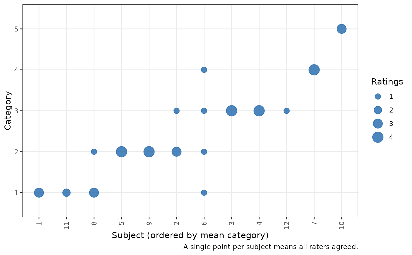
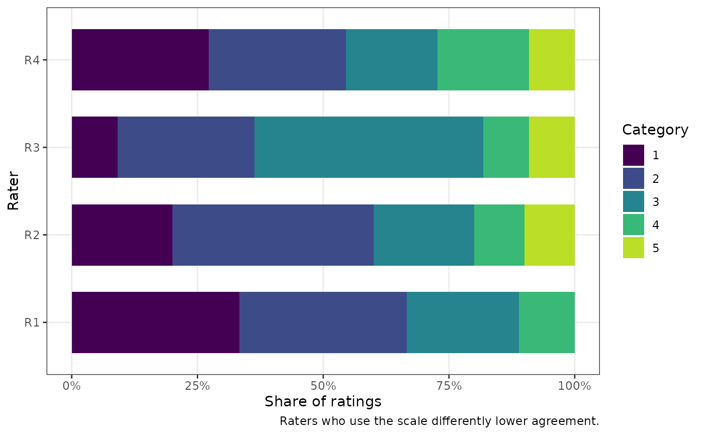
For plot(), the plot to draw: "raters" (default), the distribution of each rater's ratings over the categories, which shows raters who use the scale differently; "subjects", the ratings of each subject, with subjects ordered by their mean category, where a single large point marks complete agreement; or, for ord_kappa_test() only, "effects", each rater's estimated effect (conditional mode) on the latent scale with a 95% interval, where positive values mark raters who give higher ratings.

Value

summary

An object of class summary.cac_htest: a list with the description in text, the style used, the S-value (s.value, when there is a p-value) and the parts used to build it. It prints as a paragraph.

plot

A ggplot2 plot (see type).

Examples

ratings <- data.frame(
  R1 = c(1, 2, 3, 3, 2, 1, 4, 1, 2, NA, NA, NA),
  R2 = c(1, 2, 3, 3, 2, 2, 4, 1, 2, 5, NA, NA),
  R3 = c(NA, 3, 3, 3, 2, 3, 4, 2, 2, 5, 1, 3),
  R4 = c(1, 2, 3, 3, 2, 4, 4, 1, 2, 5, 1, NA))
res <- cac_test(col.names = c("R1", "R2", "R3", "R4"), data = ratings,
                null.value = 0.4, alternative = "greater")
summary(res)
#> The test is statistically significant (t(11) = 2.63, p = 0.012; Gwet's
#> AC1 = 0.775, 95% lower bound 0.519) at the 0.05 alpha level. The null
#> hypothesis can be rejected: at the desired error rate, it can be stated
#> that the true Gwet's AC1 is greater than 0.4. The estimate is Gwet's
#> AC1: agreement corrected for the chance that a rater classifies at
#> random (Gwet, 2008) (observed agreement 0.818, chance agreement 0.190).
#> Only identical ratings counted as agreement. The data had 12 subjects,
#> of whom 1 had a single rating, rated by 4 raters (41 ratings) in 5
#> categories. The interval and t test use the standard error of Gwet
#> (2008), which treats the subjects as a random sample and the raters as
#> fixed, with 11 degrees of freedom.
summary(res, style = "estimation")
#> The estimated Gwet's AC1 was 0.775 (95% lower compatibility bound
#> 0.519). Values above this bound are the most compatible with the data,
#> given the model and its assumptions. Against the hypothesis that the
#> true Gwet's AC1 is at most 0.4, p = 0.012, an S-value of 6.41 bits of
#> information (S = -log2 p): about as surprising as getting 6 heads in a
#> row from 6 tosses of a fair coin. The estimate is Gwet's AC1: agreement
#> corrected for the chance that a rater classifies at random (Gwet, 2008)
#> (observed agreement 0.818, chance agreement 0.190). Only identical
#> ratings counted as agreement. The data had 12 subjects, of whom 1 had a
#> single rating, rated by 4 raters (41 ratings) in 5 categories. The
#> interval and t test use the standard error of Gwet (2008), which treats
#> the subjects as a random sample and the raters as fixed, with 11
#> degrees of freedom.
plot(res)

plot(res, type = "subjects")