Plot Correlation Coefficients
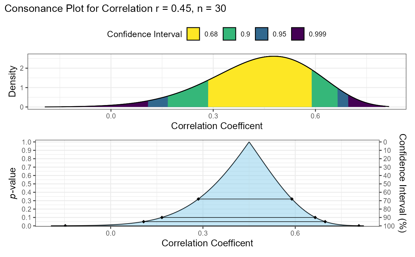
plot_cor.RdCreates consonance plots (confidence curves and/or consonance density functions) for correlation coefficients, allowing visualization of uncertainty around correlation estimates.
Arguments
- r
The observed correlation coefficient.
- n
Total number of observations (sample size).
- method
The method by which the coefficient was calculated:
"pearson": Pearson's product-moment correlation (default)
"spearman": Spearman's rank correlation
"kendall": Kendall's tau
- type
Choose which plot(s) to create:
"c": consonance function only (p-values across potential parameter values)
"cd": consonance density function only (distribution of plausible parameter values)
c("c", "cd"): both plots together (default)
- levels
Numeric vector of confidence levels to display (default: c(.68, .9, .95, .999)). These correspond to the confidence intervals shown on the plot.
Details
Consonance plots provide a graphical representation of the full range of confidence intervals for correlation coefficients at different confidence levels. These plots help visualize the uncertainty around correlation estimates and go beyond the traditional approach of reporting only a single confidence interval (typically 95%).
The function creates two types of visualizations:
Consonance function ("c"): Shows how p-values change across different possible values of the correlation coefficient. The x-axis represents possible correlation values, and the y-axis represents the corresponding p-values from two-sided hypothesis tests.
Consonance density ("cd"): Shows the distribution of plausible values for the correlation coefficient. This can be interpreted as showing where the "weight of evidence" is concentrated.
These plots are particularly useful for:
Visualizing uncertainty around correlation estimates
Understanding the precision of correlation estimates
Comparing the relative plausibility of different correlation values
Going beyond the binary "significant vs. non-significant" interpretation
These types of plots are discussed by Schweder & Hjort (2016) and Rafi & Greenland (2020).
References
Schweder, T., & Hjort, N. L. (2016). Confidence, likelihood, probability: Statistical inference with confidence distributions. Cambridge University Press. ISBN: 9781316445051
Rafi, Z., & Greenland, S. (2020). Semantic and cognitive tools to aid statistical science: Replace confidence and significance by compatibility and surprise. BMC Medical Research Methodology, 20, 244. doi:10.1186/s12874-020-01105-9
See also
Other Correlations:
boot_cor_test(),
corsum_test(),
power_z_cor(),
z_cor_test()
Other plotting functions:
plot_pes(),
plot_smd()
Examples
# Example 1: Basic consonance plot for Pearson correlation
# For a correlation of r = 0.45 with n = 30
plot_cor(r = 0.45, n = 30)

# Example 2: Consonance function only for Spearman correlation
plot_cor(r = 0.6, n = 25, method = "spearman", type = "c")

# Example 3: Consonance density only for Kendall's tau
plot_cor(r = 0.3, n = 40, method = "kendall", type = "cd")

# Example 4: Custom confidence levels
plot_cor(r = 0.5, n = 50, levels = c(0.5, 0.8, 0.95))

# Example 5: Saving and further customizing the plot
library(ggplot2)
p <- plot_cor(r = 0.45, n = 30)
p + theme_minimal() +
  labs(title = "Consonance Plot for Correlation r = 0.45, n = 30")
