Chapter 6 Power for Three-way Interactions

There are almost no software solutions that allow researchers to perform power anaysis for more complex designs. Through simulation, it is relatively straightforward to examine the power for designs with multiple factors with many levels.

Let’s start with a 2x2x2 between-subjects design. We collect 50 participants in each between participant condition (so 400 participants in total - \(50(n)\times2(levels)\times2(levels)\times2(levels)= 400\)).

# With 2x2x2 designs, 
# the names for paired comparisons can become very long. 
# So here I abbreviate terms: 
#   Size, Color, and Cognitive Load, have values:
# b = big, s = small, g = green, 
# r = red, pres = present, abs = absent.  
labelnames <- c("Size", "b", "s", "Color", "g", "r", 
                "Load", "pres", "abs") #
design_result <- ANOVA_design(design = "2b*2b*2b", 
                              #sample size per group 
                              n = 50, 
                              #pattern of means
                              mu = c(2, 2, 6, 1, 6, 6, 1, 8), 
                              sd = 10, #standard deviation
                              labelnames = labelnames)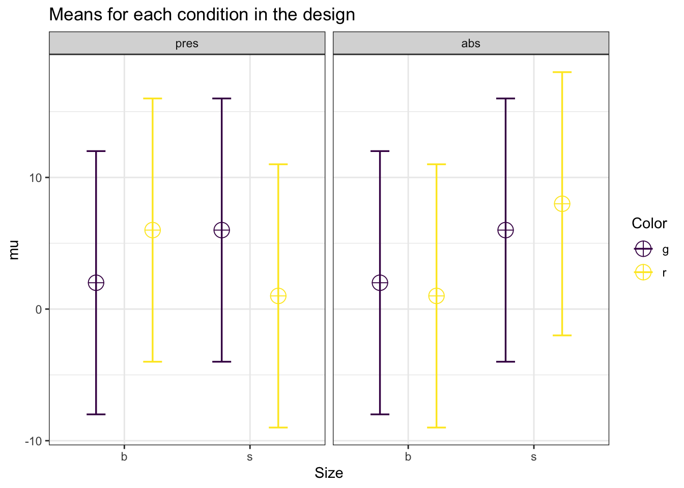 

simulation_result <- ANOVA_power(design_result, 
                                 alpha_level = alpha_level, 
                                 nsims = nsims,
                                 verbose = FALSE)

Table 6.1: Simulated ANOVA Result

	power	effect_size
anova_Size	70.17	0.0179159
anova_Color	4.86	0.0025370
anova_Load	8.31	0.0032647
anova_Size:Color	31.89	0.0081783
anova_Size:Load	85.45	0.0248185
anova_Color:Load	7.80	0.0031794
anova_Size:Color:Load	85.60	0.0248853

exact_result <- ANOVA_exact(design_result,
                            alpha_level = alpha_level,
                            verbose = FALSE)

Table 6.2: Exact ANOVA Result

	power	partial_eta_squared	cohen_f	non_centrality
Size	70.330132	0.0156937	0.1262691	6.25
Color	5.000000	0.0000000	0.0000000	0.00
Load	7.895322	0.0006373	0.0252538	0.25
Size:Color	32.172729	0.0057070	0.0757614	2.25
Size:Load	84.912313	0.0224439	0.1515229	9.00
Color:Load	7.895322	0.0006373	0.0252538	0.25
Size:Color:Load	84.912313	0.0224439	0.1515229	9.00

#Analytical power calculation
power_analytic <- power_threeway_between(design_result)
power_analytic$power_A

## [1] 70.33333

power_analytic$power_B

## [1] 5

power_analytic$power_C

## [1] 7.895539

power_analytic$power_AB

## [1] 32.17471

power_analytic$power_AC

## [1] 84.91491

power_analytic$power_BC

## [1] 7.895539

power_analytic$power_ABC

## [1] 84.91491

power_analytic$eta_p_2_A

## [1] 0.01538462

power_analytic$eta_p_2_B

## [1] 0

power_analytic$eta_p_2_C

## [1] 0.0006246096

power_analytic$eta_p_2_AB

## [1] 0.005593536

power_analytic$eta_p_2_AC

## [1] 0.02200489

power_analytic$eta_p_2_BC

## [1] 0.0006246096

power_analytic$eta_p_2_ABC

## [1] 0.02200489

We can also confirm the power analysis in g*power (Faul et al. 2007). g*power allows you to compute the power for a three-way interaction - if you know the Cohen’s f value to enter. Cohen’s f is calculated based on the means for the interaction, the sum of squares of the effect, and the sum of squares of the errors. This is quite a challenge by hand, but we can simulate the results, or use the analytical solution we programmed to get Cohen’s f for the pattern of means that we specified.

# The power for the AC interaction (Size x Load) is 0.873535. 
power_analytic$power_AC

## [1] 84.91491

# We can enter the Cohen's f for this interaction. 
power_analytic$Cohen_f_AC

## [1] 0.15

# We can double check the calculated lambda
power_analytic$lambda_AC

## [1] 9

# We can double check the critical F value
power_analytic$F_critical_AC

## [1] 3.864929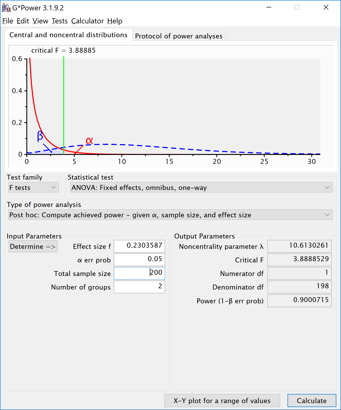

A three-way ANOVA builds on the same principles as a one-way ANOVA. We look at whether the differences between groups are large, compared to the standard deviation. For the main effects we simply have 2 groups of 200 participants, and 2 means. If the population standard deviations are identical across groups, this is not in any way different from a one-way ANOVA. Indeed, we can show this by simulating a one-way ANOVA, where instead of 8 conditions, we have two conditions, and we average over the 4 groups of the other two factors. For example, for the main effect of size above can be computed analytically. There might be a small difference in the degrees of freedom of the two tests, or it is just random variation (And it will disappear when the number of iterations in the simulation, nsim, is increased).

string <- "2b"
n <- 200
mu <- c(mean(c(2, 2, 6, 1)), mean(c(6, 6, 1, 8)))
sd <- 10
labelnames <- c("Size", "big", "small")
design_result <- ANOVA_design(design = string,
                   n = n, 
                   mu = mu, 
                   sd = sd, 
                   labelnames = labelnames)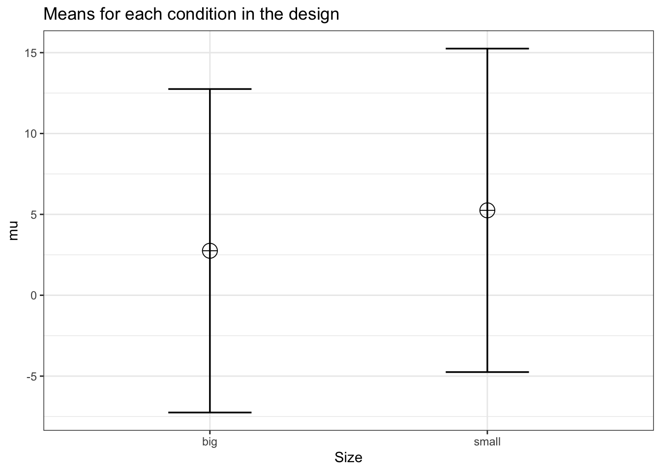

simulation_result <- ANOVA_power(design_result, 
                                 alpha_level = alpha_level, 
                                 nsims = nsims,
                                 verbose = FALSE)

Table 6.3: Simulated ANOVA Result

	power	effect_size
anova_Size	69.63	0.0177096

exact_result <- ANOVA_exact(design_result,
                            alpha_level = alpha_level,
                            verbose = FALSE)

Table 6.4: Exact ANOVA Result

	power	partial_eta_squared	cohen_f	non_centrality
Size	70.33333	0.0154607	0.1253137	6.25

# Power based on analytical solution
power_oneway_between(design_result)$power 

## [1] 70.33333

Similarly, we can create a 2 factor design where we average over the third factor, and recreate the power analysis for the Two-Way interaction. For example, we can group over the Cognitive Load condition, and look at the Size by Color Interaction:

string <- "2b*2b"
n <- 100
mu <- c(mean(c(1, 1)), mean(c(6, 1)), mean(c(6, 6)), mean(c(1, 6)))
sd <- 10
labelnames <- c("Size", "big", "small", "Color", "green", "red")
design_result <- ANOVA_design(design = string,
                   n = n, 
                   mu = mu, 
                   sd = sd, 
                   labelnames = labelnames)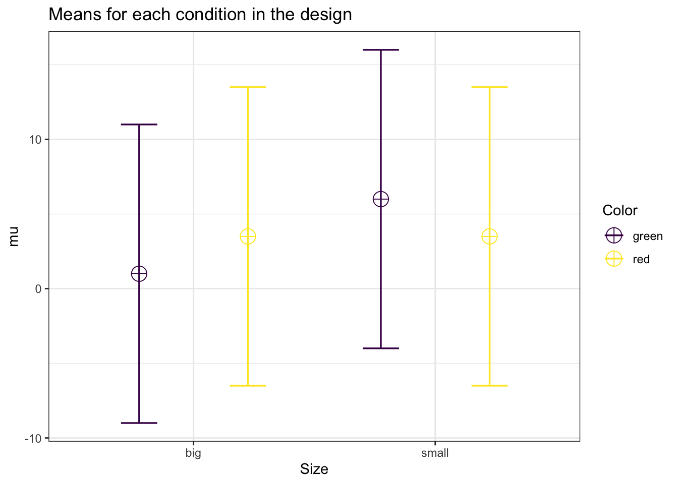

simulation_result <- ANOVA_power(design_result, 
                                 alpha_level = alpha_level, 
                                 nsims = nsims,
                                 verbose = FALSE)

Table 6.5: Simulated ANOVA Result

	power	effect_size
anova_Size	70.41	0.0179067
anova_Color	5.10	0.0025282
anova_Size:Color	70.80	0.0179360

exact_result <- ANOVA_exact(design_result,
                            alpha_level = alpha_level,
                            verbose = FALSE)

Table 6.6: Exact ANOVA Result

	power	partial_eta_squared	cohen_f	non_centrality
Size	70.33227	0.0155376	0.1256297	6.25
Color	5.00000	0.0000000	0.0000000	0.00
Size:Color	70.33227	0.0155376	0.1256297	6.25

# Power based on analytical solution
power_res <- power_twoway_between(design_result) 
power_res$power_A

## [1] 70.33228

power_res$power_B

## [1] 5

power_res$power_AB

## [1] 70.33228

string <- "2b*2b*2b"
n <- 50
mu <- c(5, 3, 2, 6, 1, 4, 3, 1) 
sd <- 10
r <- 0.0
labelnames <- c("Size", "big", "small", 
                "Color", "green", "red", 
                "CognitiveLoad", "present", "absent") 
design_result <- ANOVA_design(design = string,
                   n = n, 
                   mu = mu, 
                   sd = sd, 
                   labelnames = labelnames)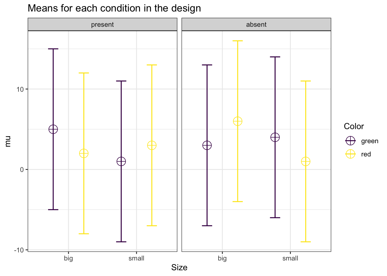

simulation_result <- ANOVA_power(design_result, 
                                 alpha_level = alpha_level, 
                                 nsims = nsims,
                                 verbose = FALSE)

Table 6.7: Simulated ANOVA Result

	power	effect_size
anova_Size	41.15	0.0101529
anova_Color	5.97	0.0027337
anova_CognitiveLoad	11.55	0.0039201
anova_Size:Color	5.67	0.0027030
anova_Size:CognitiveLoad	5.45	0.0026596
anova_Color:CognitiveLoad	5.54	0.0027225
anova_Size:Color:CognitiveLoad	78.61	0.0214761

exact_result <- ANOVA_exact(design_result,
                            alpha_level = alpha_level,
                            verbose = FALSE)

Table 6.8: Exact ANOVA Result

	power	partial_eta_squared	cohen_f	non_centrality
Size	41.52809	0.0077519	0.0883883	3.0625
Color	5.71548	0.0001594	0.0126269	0.0625
CognitiveLoad	11.61777	0.0014329	0.0378807	0.5625
Size:Color	5.71548	0.0001594	0.0126269	0.0625
Size:CognitiveLoad	5.71548	0.0001594	0.0126269	0.0625
Color:CognitiveLoad	5.71548	0.0001594	0.0126269	0.0625
Size:Color:CognitiveLoad	78.32737	0.0189270	0.1388960	7.5625

#Analytical power calculation
power_analytic <- power_threeway_between(design_result)
power_analytic$power_A

## [1] 41.5306

power_analytic$power_B

## [1] 5.715533

power_analytic$power_C

## [1] 11.61827

power_analytic$power_AB

## [1] 5.715533

power_analytic$power_AC

## [1] 5.715533

power_analytic$power_BC

## [1] 5.715533

power_analytic$power_ABC

## [1] 78.33036

power_analytic$eta_p_2_A

## [1] 0.007598077

power_analytic$eta_p_2_B

## [1] 0.0001562256

power_analytic$eta_p_2_C

## [1] 0.001404275

power_analytic$eta_p_2_AB

## [1] 0.0001562256

power_analytic$eta_p_2_AC

## [1] 0.0001562256

power_analytic$eta_p_2_BC

## [1] 0.0001562256

power_analytic$eta_p_2_ABC

## [1] 0.01855544

The power for interactions depends on Cohen’s f, the alpha level, the sample size, and the degrees of freedom.

# With 2x2x2 designs, 
# the names for paired comparisons can become very long. 
# So here the sample size abbreviate terms
# Size, Color, and Cognitive Load, have values:
# b = big, s = small, g = green, 
# r = red, pres = present, abs = absent.  
labelnames <- c("Size", "b", "s", "x", "Color", "g", "r", 
                "Load", "pres", "abs") #
design_result <- ANOVA_design(design = "3b*2b*2b", 
                              n = 15, 
                              mu = c(20, 0, 0, 0, 0, 
                                     0, 0, 0, 0, 0, 0, 20), 
                              
                              sd = 20, 
                              labelnames = labelnames)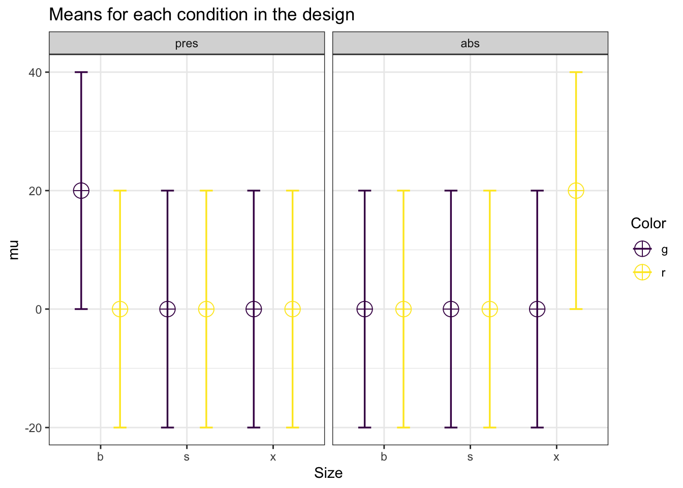 

# Power based on exact simulations
exact_result <- ANOVA_exact(design_result,
                            verbose = FALSE)

Table 6.9: Exact ANOVA Result

	power	partial_eta_squared	cohen_f	non_centrality
Size	26.92604	0.0146628	0.1219875	2.5
Color	5.00000	0.0000000	0.0000000	0.0
Load	5.00000	0.0000000	0.0000000	0.0
Size:Color	67.93217	0.0427350	0.2112886	7.5
Size:Load	67.93217	0.0427350	0.2112886	7.5
Color:Load	60.38579	0.0289017	0.1725164	5.0
Size:Color:Load	26.92604	0.0146628	0.1219875	2.5

#Analytical power calculation
power_analytic <- power_threeway_between(design_result)
power_analytic$power_A

## [1] 5

power_analytic$power_B

## [1] 5

power_analytic$power_C

## [1] 48.6496

power_analytic$power_AB

## [1] 34.7961

power_analytic$power_AC

## [1] 67.97466

power_analytic$power_BC

## [1] 91.55713

power_analytic$power_ABC

## [1] NaN

power_analytic$eta_p_2_A

## [1] 0

power_analytic$Cohen_f_A

## [1] 0

We see that a pattern of means of 0, 0, 0, 0, 0, 0, 0, 20 for a 2x2x2 interaction equals a Cohen’s f of 0.25.

labelnames <- c("Size", "b", "s", "Color", "g", "r")
design_result <- ANOVA_design(design = "2b*2b", 
                              n = 10, 
                              mu = c(0, 0, 0, 10), 
                              sd = 10, 
                              labelnames = labelnames)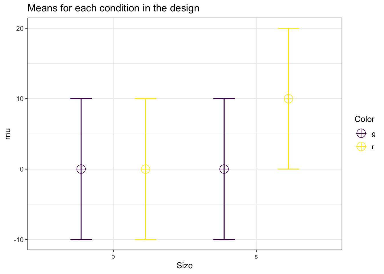 

# Power based on exact simulations
exact_result <- ANOVA_exact(design_result,
                            verbose = FALSE)

Table 6.10: Exact ANOVA Result

	power	partial_eta_squared	cohen_f	non_centrality
Size	33.71329	0.0649351	0.2635231	2.5
Color	33.71329	0.0649351	0.2635231	2.5
Size:Color	33.71329	0.0649351	0.2635231	2.5

#Analytical power calculation
power_analytic <- power_twoway_between(design_result)
power_analytic$power_A

## [1] 33.71329

power_analytic$eta_p_2_A

## [1] 0.05882353

power_analytic$Cohen_f_A

## [1] 0.25

Cohen’s f is twice as large for a 2x2 design with the same mean value in one of four cells. In a 2 factor between design.

labelnames <- c("Size", "b", "s")
design_result <- ANOVA_design(design = "2b", 
                              n = 10,  
                              mu = c(0, 5), 
                              sd = 10, 
                              labelnames = labelnames)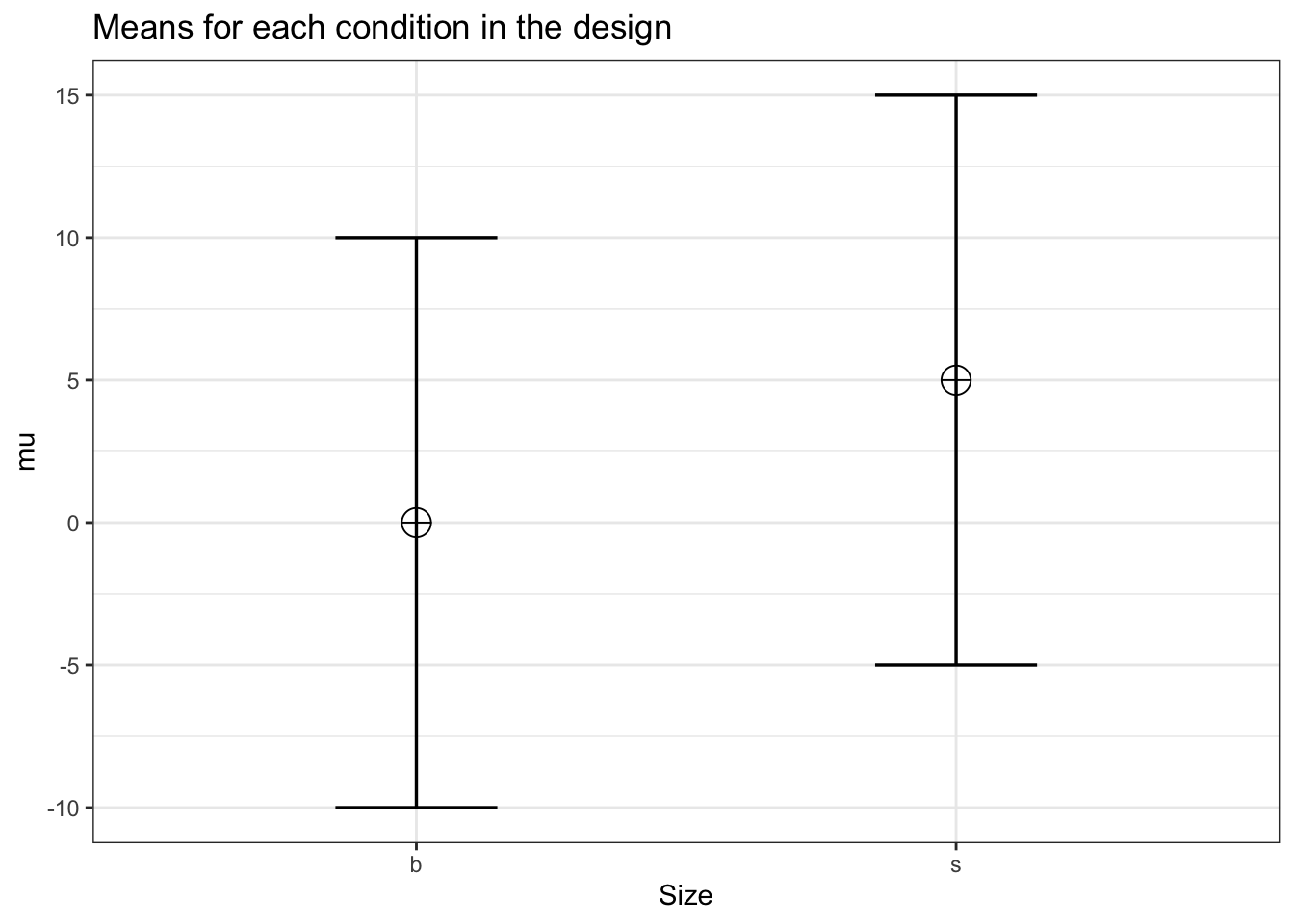 

# Power based on exact simulations
exact_result <- ANOVA_exact(design_result,
                            verbose = FALSE)

Table 6.11: Exact ANOVA Result

	power	partial_eta_squared	cohen_f	non_centrality
Size	18.50957	0.0649351	0.2635231	1.25

#Analytical power calculation
power_analytic <- power_oneway_between(design_result)
power_analytic$power

## [1] 18.50957

power_analytic$eta_p_2

## [1] 0.05882353

power_analytic$Cohen_f

## [1] 0.25

References

Faul, Franz, Edgar Erdfelder, Albert-Georg Lang, and Axel Buchner. 2007. “G*power 3: A Flexible Statistical Power Analysis Program for the Social, Behavioral, and Biomedical Sciences.” Behavior Research Methods 39 (2): 175–91. http://www.psychologie.hhu.de/arbeitsgruppen/allgemeine-psychologie-und-arbeitspsychologie/gpower.html.