Chapter 10 Analytic Power Functions

For some designs it is possible to calculate power analytically, using closed functions. Within the Superpower package we have included a number of these closed functions. As you will see below, each analytic function only serves a very narrow scenario while the simulations functions are much more flexible. In addition, we will compare these functions to other packages/software. Please note, that the analytic power functions are designed to reject designs that are not appropriate for the functions (i.e., a 3w design will be rejected by the power_oneway_between function).

10.1 One-Way Between Subjects ANOVA

First, we can setup a one-way design with four levels, and perform a exact simulation power analysis with the ANOVA_exact function.

string <- "4b"
n <- 60
mu <- c(80, 82, 82, 86) 

# Enter means in the order that matches the labels below.
sd <- 10
design_result <- ANOVA_design(design = string,
                   n = n, 
                   mu = mu, 
                   sd = sd)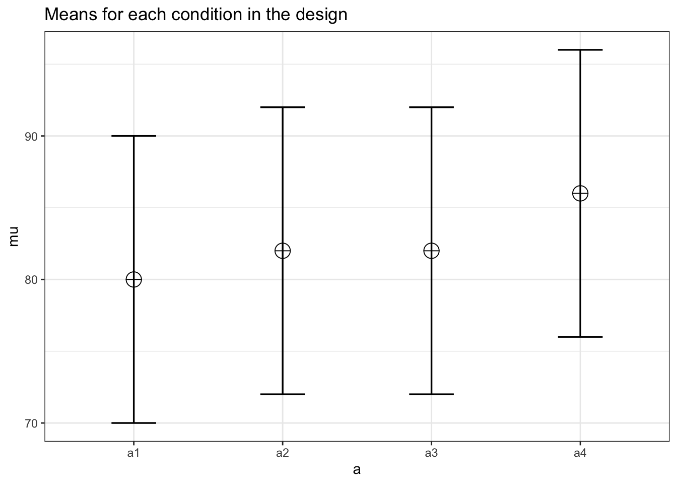

exact_result <- ANOVA_exact(design_result,
                            alpha_level = alpha_level,
                            verbose = FALSE)

Table 10.1: Exact ANOVA Result

	power	partial_eta_squared	cohen_f	non_centrality
a	81.21291	0.0460792	0.2197842	11.4

We can also calculate power analytically with a Superpower function.

#using default alpha level of .05
power_oneway_between(design_result)$power 

## [1] 81.21291

This is a generalized function for one-way ANOVA’s for any number of groups. It is in part based on code from the pwr2ppl (Aberson 2020) package (but Aberson’s code allows for different n per condition, and different sd per condition).

pwr2ppl::anova1f_4(m1 = 80, m2 = 82, m3 = 82, m4 = 86,
          s1 = 10, s2 = 10, s3 = 10, s4 = 10,
          n1 = 60, n2 = 60, n3 = 60, n4 = 60,
          alpha = .05)

## Power  = 0.812 for eta-squared = 0.05

We can also use the function in the pwr package (Champely 2020). Note that we need to calculate f to use this function, which is based on the means and sd, as illustrated in the formulas above.

pwr::pwr.anova.test(n = 60,
               k = 4,
               f = 0.2179449,
               sig.level = 0.05)

## 
##      Balanced one-way analysis of variance power calculation 
## 
##               k = 4
##               n = 60
##               f = 0.2179449
##       sig.level = 0.05
##           power = 0.8121289
## 
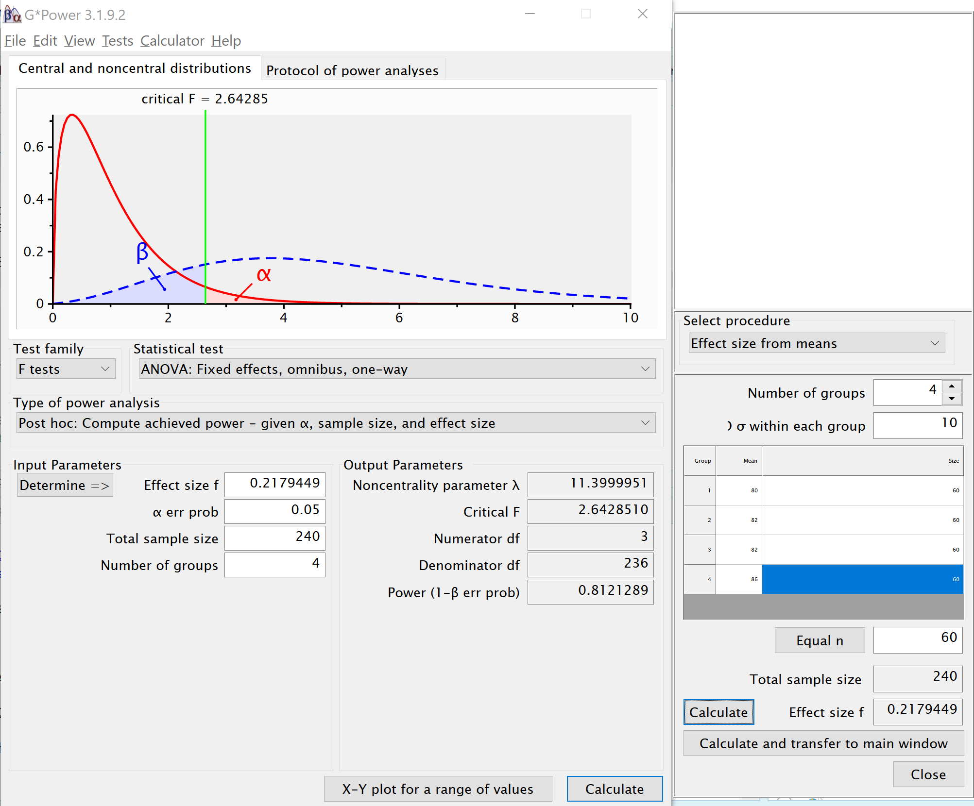
## NOTE: n is number in each group

Finally, g*Power (Faul et al. 2007) provides the option to calculate f from the means, sd and n for the cells. It can then be used to calculate power.

10.2 Two-way Between Subject Interaction

Now, we will setup a 2x2 between-subject ANOVA.

string <- "2b*2b"
n <- 20
mu <- c(20, 20, 20, 25) 
# Enter means in the order that matches the labels below.
sd <- 5

design_result <- ANOVA_design(design = string,
                   n = n, 
                   mu = mu, 
                   sd = sd)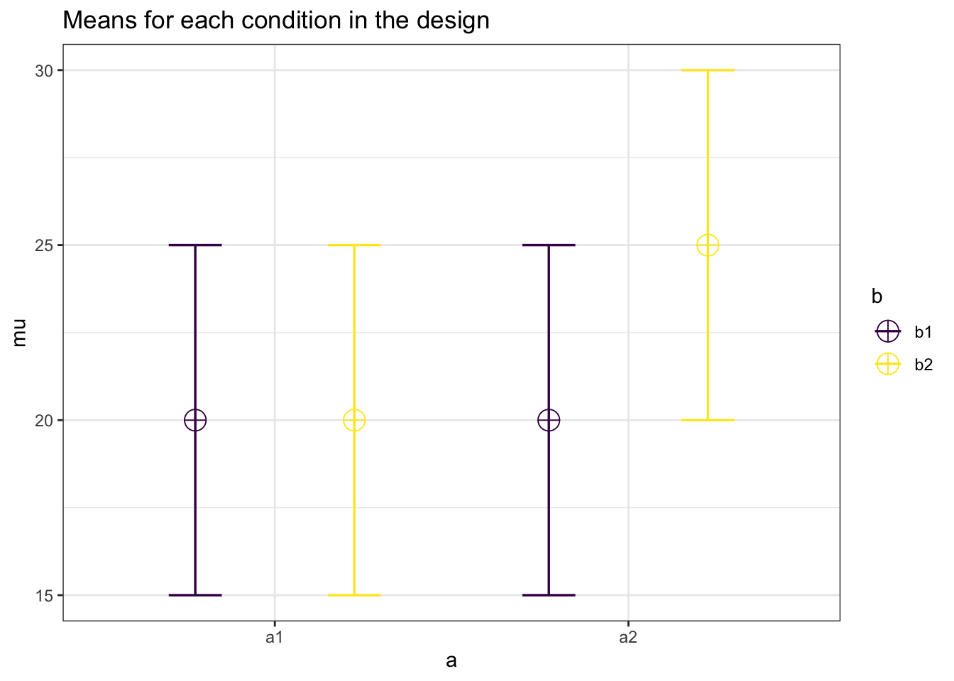

exact_result <- ANOVA_exact(design_result,
                            alpha_level = alpha_level,
                            verbose = FALSE)

Table 10.2: Exact ANOVA Result

	power	partial_eta_squared	cohen_f	non_centrality
a	59.78655	0.0617284	0.2564946	5
b	59.78655	0.0617284	0.2564946	5
a:b	59.78655	0.0617284	0.2564946	5

Now, let’s use the analytic function power_twoway_between.

#using default alpha level of .05
power_res <- power_twoway_between(design_result) 
power_res$power_A

## [1] 59.78655

power_res$power_B

## [1] 59.78655

power_res$power_AB

## [1] 59.78655

We can compare these results to (Aberson 2020), as well.

pwr2ppl::anova2x2(m1.1 = 20,
         m1.2 = 20,
         m2.1 = 20,
         m2.2 = 25,
         s1.1 = 5,
         s1.2 = 5,
         s2.1 = 5,
         s2.2 = 5,
         n1.1 = 20,
         n1.2 = 20,
         n2.1 = 20,
         n2.2 = 20,
         alpha = .05,
         all = "OFF")

## Power for Main Effect Factor A = 0.598

## Power for Main Effect Factor B = 0.598

## Power for Interaction AxB = 0.598

10.3 3x3 Between Subject ANOVA

We can extend this function to a two-way design with 3 levels.

string <- "3b*3b"
n <- 20
mu <- c(20, 20, 20, 20, 20, 20, 20, 20, 25) 
# Enter means in the order that matches the labels below.
sd <- 5

design_result <- ANOVA_design(design = string,
                   n = n, 
                   mu = mu, 
                   sd = sd)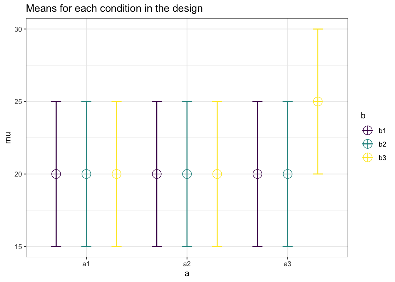

exact_result <- ANOVA_exact(design_result,
                            alpha_level = alpha_level,
                            verbose = FALSE)

Table 10.3: Exact ANOVA Result

	power	partial_eta_squared	cohen_f	non_centrality
a	44.86306	0.0253325	0.1612169	4.444444
b	44.86306	0.0253325	0.1612169	4.444444
a:b	64.34127	0.0494132	0.2279952	8.888889

#using default alpha level of .05
power_res <- power_twoway_between(design_result) 
power_res$power_A

## [1] 44.86306

power_res$power_B

## [1] 44.86306

power_res$power_AB

## [1] 64.34127

References

Aberson, Chris. 2020. Pwr2ppl: Power Analyses for Common Designs (Power to the People). https://CRAN.R-project.org/package=pwr2ppl.

Champely, Stephane. 2020. Pwr: Basic Functions for Power Analysis. https://github.com/heliosdrm/pwr.

Faul, Franz, Edgar Erdfelder, Albert-Georg Lang, and Axel Buchner. 2007. “G*power 3: A Flexible Statistical Power Analysis Program for the Social, Behavioral, and Biomedical Sciences.” Behavior Research Methods 39 (2): 175–91. http://www.psychologie.hhu.de/arbeitsgruppen/allgemeine-psychologie-und-arbeitspsychologie/gpower.html.