Chapter 8 Effect of Varying Designs on Power
Researchers might consider what the effects on the statistical power of their design is, when they add participants. Participants can be added to an additional condition, or to the existing design.
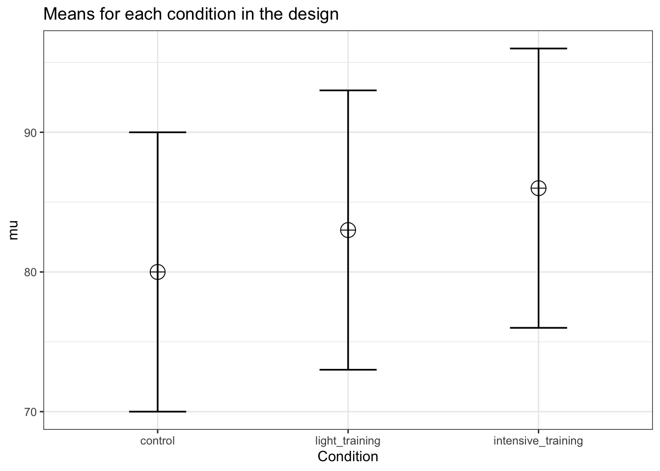
In a one-way ANOVA adding a condition means, for example, going from a 1x2 to a 1x3 design. For example, in addition to a control and intensive training condition, we add a light training condition.
string <- "2b"
n <- 50
mu <- c(80, 86)
sd <- 10
labelnames <- c("Condition", "control", "intensive_training")
design_result <- ANOVA_design(design = string,
                   n = n,
                   mu = mu,
                   sd = sd,
                   labelnames = labelnames)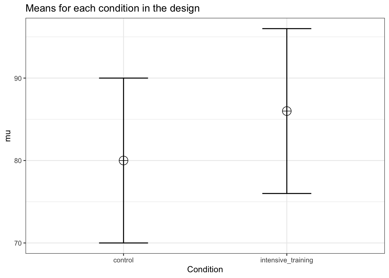
# Power for the given N in the design_result
power_oneway_between(design_result)$power
## [1] 84.38754power_oneway_between(design_result)$Cohen_f## [1] 0.3power_oneway_between(design_result)$eta_p_2## [1] 0.08256881simulation_result <- ANOVA_power(design_result,
alpha_level = alpha_level,
nsims = nsims,
verbose = FALSE)| power | effect_size | |
|---|---|---|
| anova_Condition | 84.15 | 0.0911796 |
exact_result <- ANOVA_exact(design_result,
                            alpha_level = alpha_level,
verbose = FALSE)| power | partial_eta_squared | cohen_f | non_centrality | |
|---|---|---|---|---|
| Condition | 84.38754 | 0.0841121 | 0.3030458 | 9 |
We now addd a condition. Let’s assume the ‘light training’ condition falls in between the other two means.
And we can see power across sample sizes
# Plot power curve (from 5 to 100)
plot_power(design_result, max_n = 100)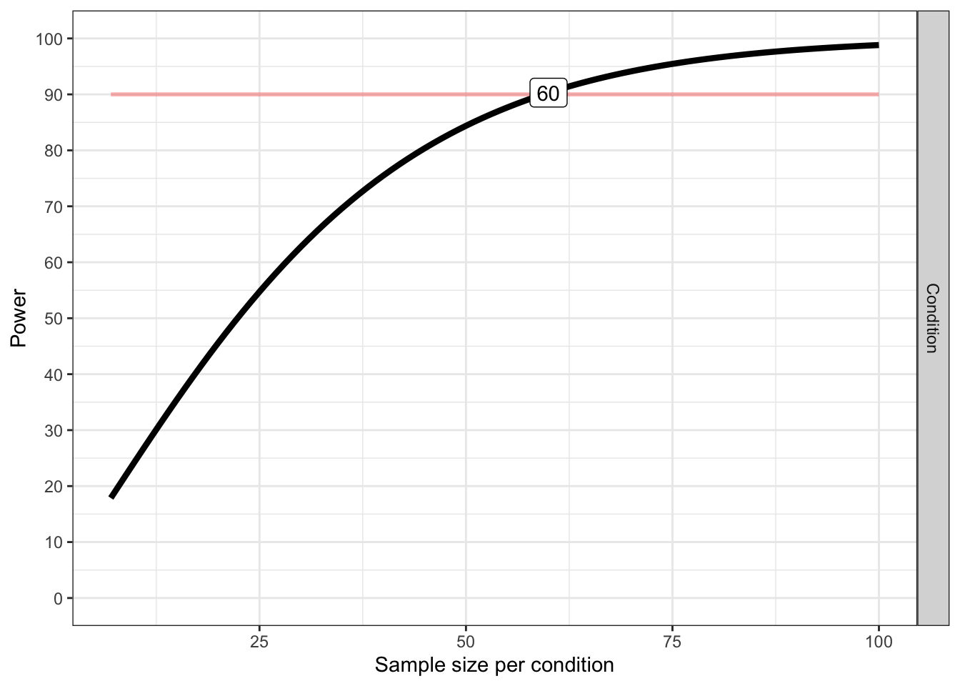
## Achieved Power and Sample Size for ANOVA-level effects
##    variable                  label  n achieved_power desired_power
## 1 Condition Desired Power Achieved 60          90.31            90
string <- "3b"
n <- 50
mu <- c(80, 83, 86)
sd <- 10
labelnames <- c("Condition", "control", "light_training", "intensive_training")
design_result <- ANOVA_design(
design = string,
n = n,
mu = mu,
sd = sd,
labelnames = labelnames
)
# Power for the given N in the design_result
power_oneway_between(design_result)$power
## [1] 76.16545power_oneway_between(design_result)$Cohen_f## [1] 0.244949power_oneway_between(design_result)$eta_p_2## [1] 0.05660377exact_result <- ANOVA_exact(design_result,
alpha_level = alpha_level,
verbose = FALSE)| power | partial_eta_squared | cohen_f | non_centrality | |
|---|---|---|---|---|
| Condition | 76.16545 | 0.0576923 | 0.2474358 | 9 |
We see that adding a condition that falls between the other two means reduces our power. Let’s instead assume that the ‘light training’ condition is not different from the control condition. In other words, the mean we add is as extreme as one of the existing means.
# Plot power curve (from 5 to 100)
plot_power(design_result, max_n = 100)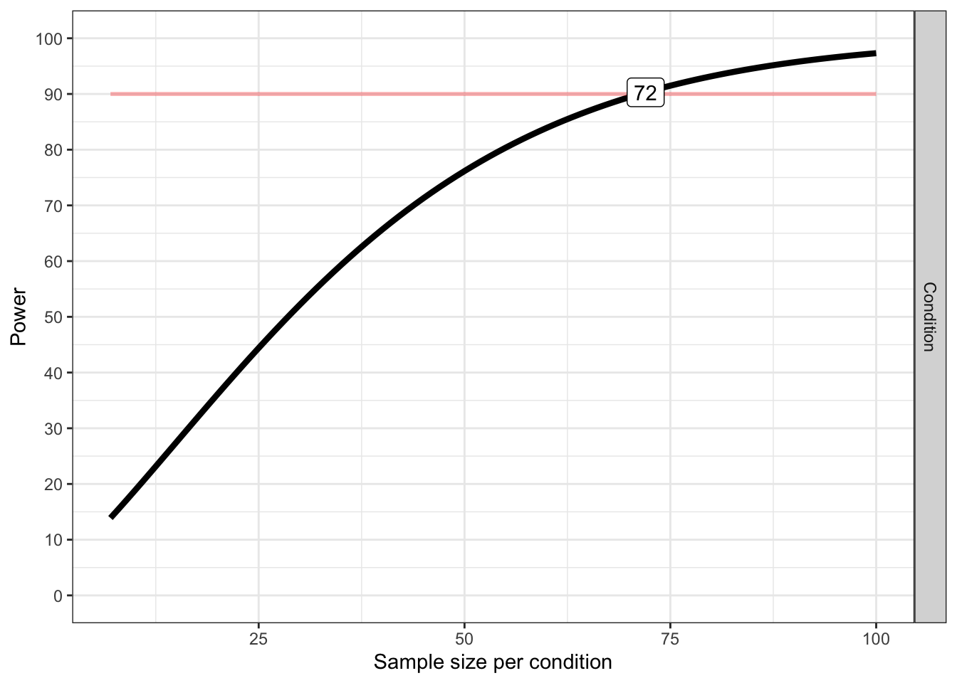
## Achieved Power and Sample Size for ANOVA-level effects
##    variable                  label  n achieved_power desired_power
## 1 Condition Desired Power Achieved 72          90.29            90
string <- "3b"
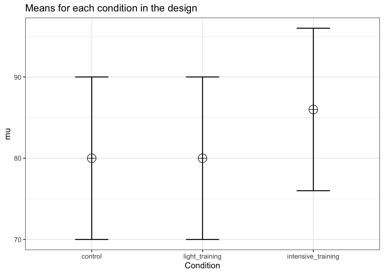
n <- 50
mu <- c(80, 80, 86)
sd <- 10
labelnames <- c("Condition", "control", "light_training", "intensive_training")
design_result <- ANOVA_design(
design = string,
n = n,
mu = mu,
sd = sd,
labelnames = labelnames
)
# Power for the given N in the design_result
power_oneway_between(design_result)$power
## [1] 87.62941power_oneway_between(design_result)$Cohen_f## [1] 0.2828427power_oneway_between(design_result)$eta_p_2## [1] 0.07407407Now power has increased. This is not always true. The power is a function of many factors in the design, incuding the effect size (Cohen’s f) and the total sample size (and the degrees of freedom and number of groups). But as we will see below, as we keep adding conditions, the power will reduce, even if initially, the power might increase.
# Plot power curve (from 5 to 100)
plot_power(design_result,max_n = 100)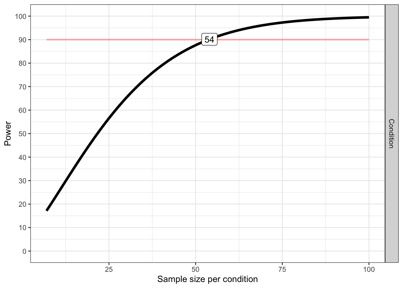
## Achieved Power and Sample Size for ANOVA-level effects
##    variable                  label  n achieved_power desired_power
## 1 Condition Desired Power Achieved 54          90.15            90
It helps to think of these different designs in terms of either partial eta-squared, or Cohen’s f (the one can easily be converted into the other).
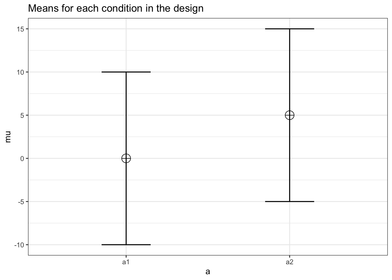
#Two groups
mu <- c(80, 86)
sd = 10
n <- 50 #sample size per condition
mean_mat <- t(matrix(mu, nrow = 2, ncol = 1)) #Create a mean matrix
# Using the sweep function to remove rowmeans from the matrix
mean_mat_res <- sweep(mean_mat, 2, rowMeans(mean_mat))
mean_mat_res
## [,1] [,2]
## [1,] -3 3MS_a <- n * (sum(mean_mat_res ^ 2) / (2 - 1))
MS_a## [1] 900SS_A <- n * sum(mean_mat_res ^ 2)
SS_A## [1] 900MS_error <- sd ^ 2
MS_error## [1] 100SS_error <- MS_error * (n * 2)
SS_error## [1] 10000eta_p_2 <- SS_A / (SS_A + SS_error)
eta_p_2## [1] 0.08256881f_2 <- eta_p_2 / (1 - eta_p_2)
f_2## [1] 0.09Cohen_f <- sqrt(f_2)
Cohen_f## [1] 0.3#Three groups
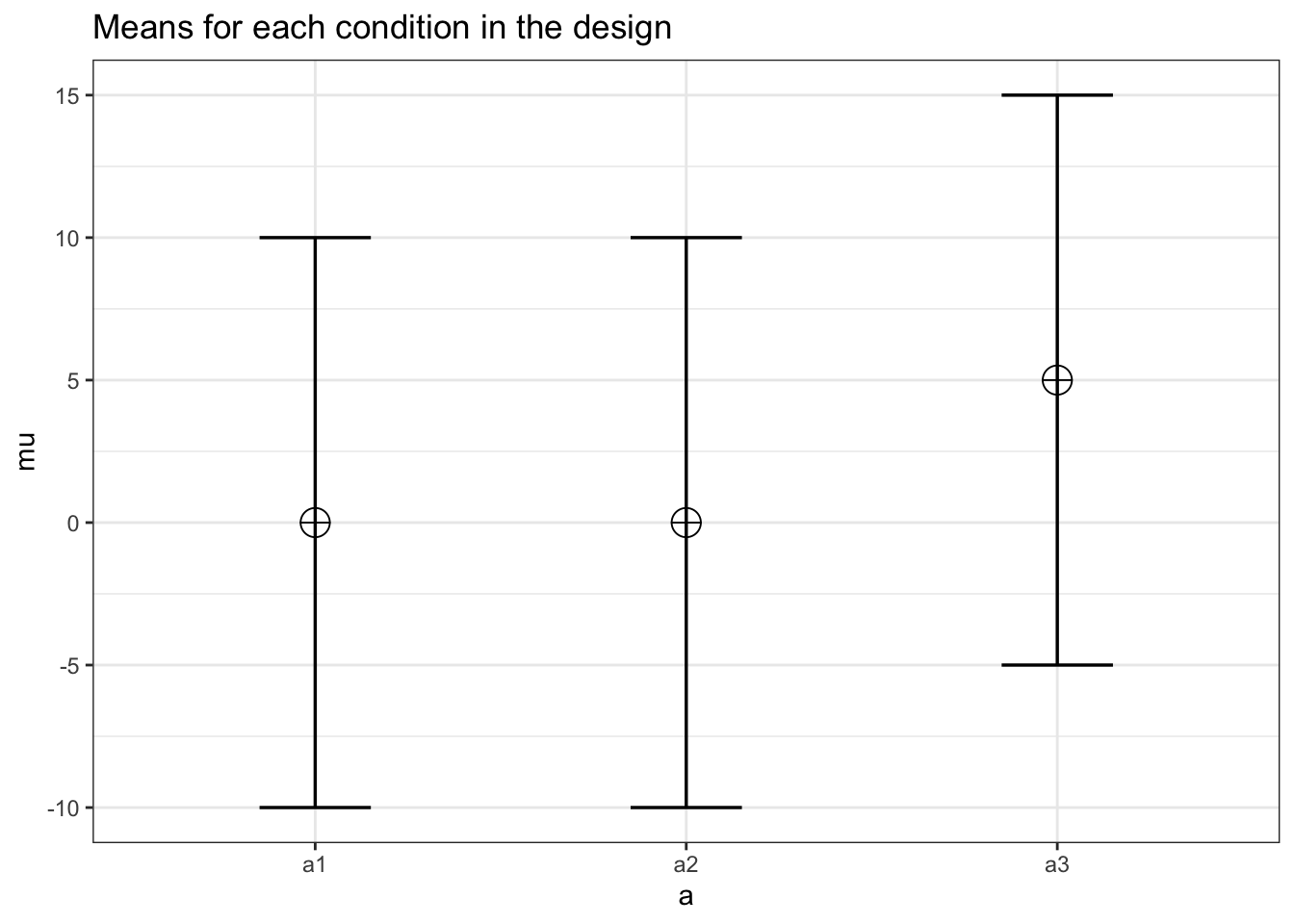
mu <- c(80, 83, 86)
sd = 10
n <- 50
mean_mat <- t(matrix(mu, nrow = 3, ncol = 1)) #Create a mean matrix
# Using the sweep function to remove rowmeans from the matrix
mean_mat_res <- sweep(mean_mat, 2, rowMeans(mean_mat))
mean_mat_res## [,1] [,2] [,3]
## [1,] -3 0 3MS_a <- n * (sum(mean_mat_res ^ 2) / (3 - 1))
MS_a## [1] 450SS_A <- n * sum(mean_mat_res ^ 2)
SS_A## [1] 900MS_error <- sd ^ 2
MS_error## [1] 100SS_error <- MS_error * (n * 3)
SS_error## [1] 15000eta_p_2 <- SS_A / (SS_A + SS_error)
eta_p_2## [1] 0.05660377f_2 <- eta_p_2 / (1 - eta_p_2)
f_2## [1] 0.06Cohen_f <- sqrt(f_2)
Cohen_f## [1] 0.244949The SS_A or the sum of squares for the main effect, is 900 for two groups, and the SS_error for the error term is 10000. When we add a group, SS_A is 900, and the SS_error is 15000. Because the added condition falls exactly on the grand mean (83), the sum of squared for this extra group is 0. In other words, it does nothing to increase the signal that there is a difference between groups. However, the sum of squares for the error, which is a function of the total sample size, is increased, which reduces the effect size. So, adding a condition that falls on the grand mean reduces the power for the main effect of the ANOVA. Obviously, adding such a group has other benefits, such as being able to compare the two means to a new third condition.
We already saw that adding a condition that has a mean as extreme as one of the existing groups increases the power. Let’s again do the calculations step by step when the extra group has a mean as extreme as one of the two original conditions.
#Three groups
mu <- c(80, 80, 86)
sd = 10
n <- 50
mean_mat <- t(matrix(mu, nrow = 3, ncol = 1)) #Create a mean matrix
# Using the sweep function to remove rowmeans from the matrix
mean_mat_res <- sweep(mean_mat, 2, rowMeans(mean_mat))
mean_mat_res
## [,1] [,2] [,3]
## [1,] -2 -2 4MS_a <- n * (sum(mean_mat_res ^ 2) / (3 - 1))
MS_a## [1] 600SS_A <- n * sum(mean_mat_res ^ 2)
SS_A## [1] 1200MS_error <- sd ^ 2
MS_error## [1] 100SS_error <- MS_error * (n * 3)
SS_error## [1] 15000eta_p_2 <- SS_A / (SS_A + SS_error)
eta_p_2## [1] 0.07407407f_2 <- eta_p_2 / (1 - eta_p_2)
f_2## [1] 0.08Cohen_f <- sqrt(f_2)
Cohen_f## [1] 0.2828427We see the sum of squares of the error stays the same - 15000 - because it is only determined by the standard error and the sample size, but not by the differences in the means. This is an increase of 5000 compared to the 2 group design. The sum of squares (the second component that determines the size of partial eta-squared) increases, which increases Cohen’s f.
8.1 Within Designs
Now imagine our design described above was a within design. The means and sd remain the same. We collect 50 participants (instead of 100, or 50 per group, for the between design). Let’s first assume the two samples are completely uncorrelated.
string <- "2w"
n <- 50
mu <- c(80, 86)
sd <- 10
labelnames <- c("Condition", "control", "intensive_training") #
design_result <- ANOVA_design(
  design = string,
  n = n,
  mu = mu,
  sd = sd,
  labelnames = labelnames
)
power_oneway_within(design_result)$power## [1] 83.66436exact_result <- ANOVA_exact(design_result,
alpha_level = alpha_level,
verbose = FALSE)| power | partial_eta_squared | cohen_f | non_centrality | |
|---|---|---|---|---|
| Condition | 83.66436 | 0.1551724 | 0.4285714 | 9 |
We see power is ever so slightly less than for the between subject design. This is due to the loss in degrees of freedom, which is \(2(n-1)\) for between designs, and \(n-1\) for within designs. But as the correlation increases, the power advantage of within designs becomes stronger.
string <- "3w"
n <- 50
mu <- c(80, 83, 86)
sd <- 10
labelnames <- c("Condition", "control", "light_training", "intensive_training")
design_result <- ANOVA_design(
  design = string,
  n = n,
  mu = mu,
  sd = sd,
  labelnames = labelnames
)
power_oneway_within(design_result)$power## [1] 75.70841exact_result <- ANOVA_exact(design_result,
alpha_level = alpha_level,
verbose = FALSE)| power | partial_eta_squared | cohen_f | non_centrality | |
|---|---|---|---|---|
| Condition | 75.70841 | 0.0841121 | 0.3030458 | 9 |
When we add a a condition in a within design where we expect the mean to be identical to the grand mean, we again see that the power decreases. This similarly shows that adding a condition that equals the grand mean to a within subject design does not come for free, but has a power cost.
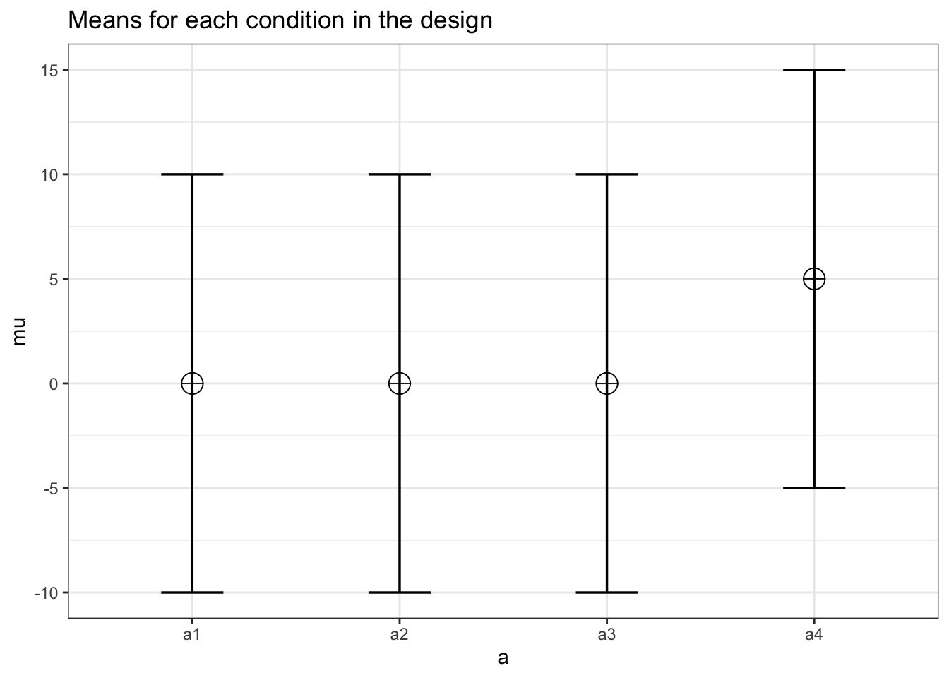
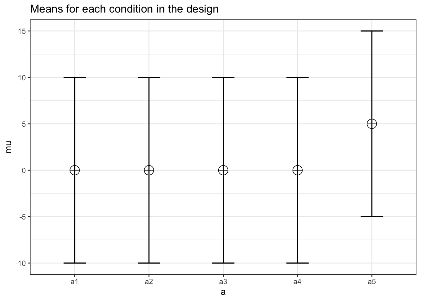
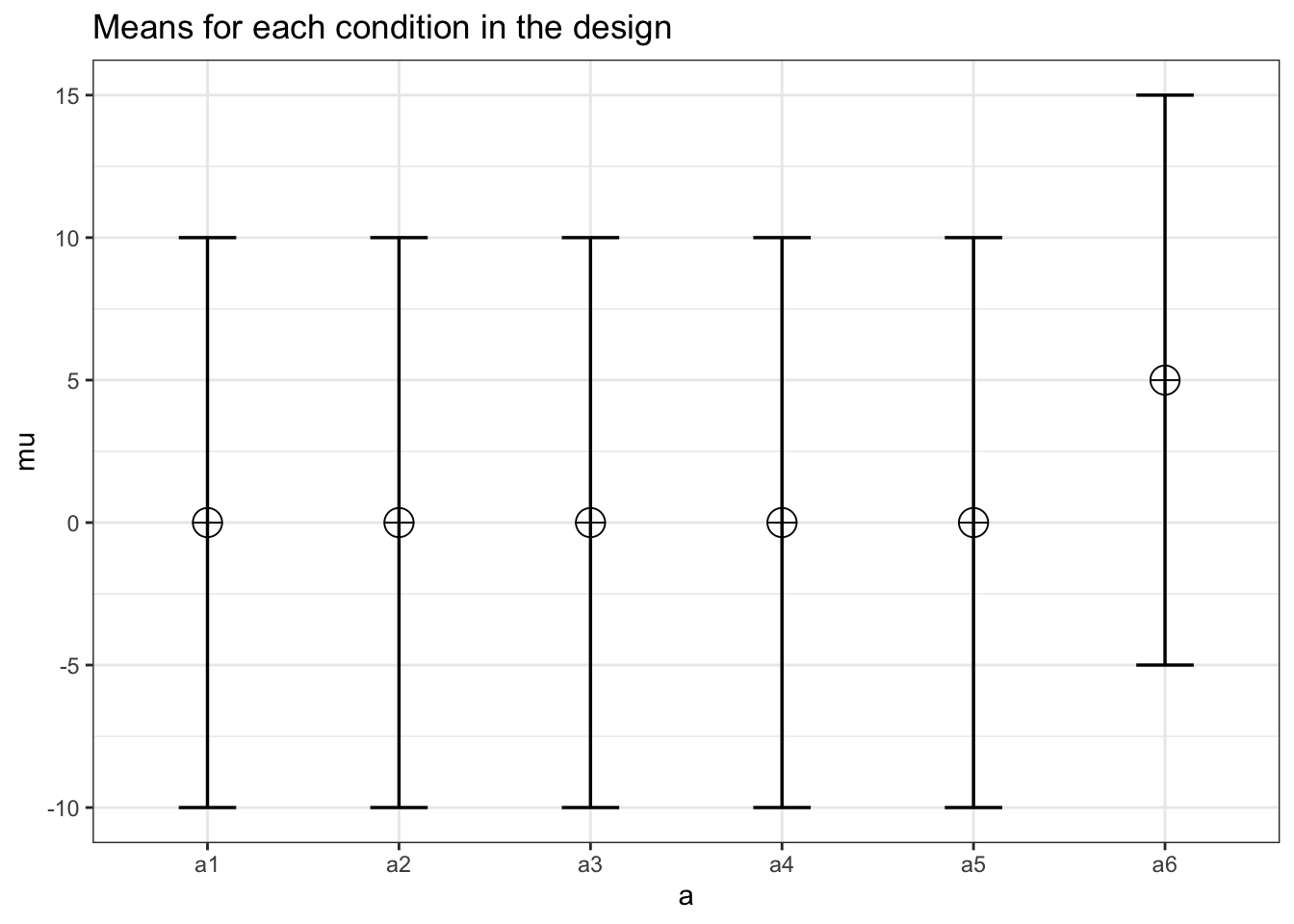
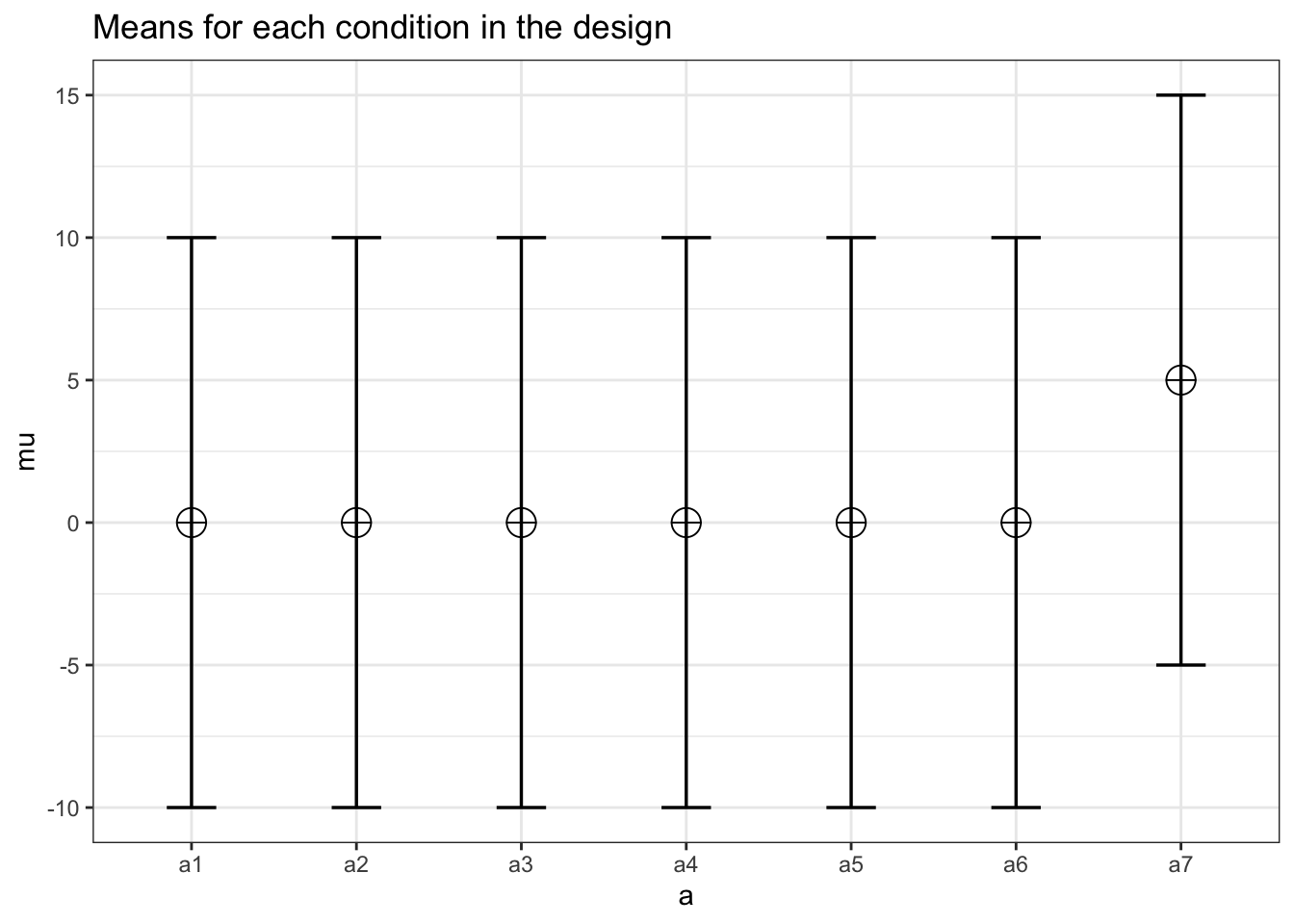
n <- 30
sd <- 10
r <- 0.5
string <- "2w"
mu <- c(0, 5)
design_result <- ANOVA_design(
  design = string,
  n = n,
  mu = mu,
  sd = sd,
  r = r
)
power_oneway_within(design_result)$power## [1] 75.39647power_oneway_within(design_result)$Cohen_f## [1] 0.25power_oneway_within(design_result)$Cohen_f_SPSS## [1] 0.5085476power_oneway_within(design_result)$lambda## [1] 7.5power_oneway_within(design_result)$F_critical## [1] 4.182964string <- "3w"
mu <- c(0, 0, 5)
design_result <- ANOVA_design(
design = string,
n = n,
mu = mu,
sd = sd,
r = r
)
power_oneway_within(design_result)$power## [1] 79.37037power_oneway_within(design_result)$Cohen_f## [1] 0.2357023power_oneway_within(design_result)$Cohen_f_SPSS## [1] 0.4152274power_oneway_within(design_result)$lambda## [1] 10power_oneway_within(design_result)$F_critical## [1] 3.155932string <- "4w"
mu <- c(0, 0, 0, 5)
design_result <- ANOVA_design(
design = string,
n = n,
mu = mu,
sd = sd,
r = r
)
power_oneway_within(design_result)$power## [1] 79.40126power_oneway_within(design_result)$Cohen_f## [1] 0.2165064power_oneway_within(design_result)$Cohen_f_SPSS## [1] 0.3595975power_oneway_within(design_result)$lambda## [1] 11.25power_oneway_within(design_result)$F_critical## [1] 2.709402string <- "5w"
mu <- c(0, 0, 0, 0, 5)
design_result <- ANOVA_design(
design = string,
n = n,
mu = mu,
sd = sd,
r = r
)
power_oneway_within(design_result)$power## [1] 78.38682power_oneway_within(design_result)$Cohen_f## [1] 0.2power_oneway_within(design_result)$Cohen_f_SPSS## [1] 0.3216338power_oneway_within(design_result)$lambda## [1] 12power_oneway_within(design_result)$F_critical## [1] 2.44988string <- "6w"
mu <- c(0, 0, 0, 0, 0, 5)
design_result <- ANOVA_design(
design = string,
n = n,
mu = mu,
sd = sd,
r = r
)
power_oneway_within(design_result)$power## [1] 76.99592power_oneway_within(design_result)$Cohen_f## [1] 0.186339power_oneway_within(design_result)$Cohen_f_SPSS## [1] 0.2936101power_oneway_within(design_result)$lambda## [1] 12.5power_oneway_within(design_result)$F_critical## [1] 2.276603string <- "7w"
mu <- c(0, 0, 0, 0, 0, 0, 5)
design_result <- ANOVA_design(
design = string,
n = n,
mu = mu,
sd = sd,
r = r
)
print(paste0("power: ", power_oneway_within(design_result)$power, "\nCohen's F: ", power_oneway_within(design_result)$Cohen_f,
             "\nCohen's F (SPSS): ", power_oneway_within(design_result)$Cohen_f_SPSS,
             "\nlambda: ", power_oneway_within(design_result)$lambda,
             "\nCritical F: ",
             power_oneway_within(design_result)$F_critical
             ))
## [1] "power: 75.4600950274594\nCohen's F: 0.174963553055941\nCohen's F (SPSS): 0.271830141109781\nlambda: 12.8571428571429\nCritical F: 2.15101618343483"# power_oneway_within(design_result)$power
# power_oneway_within(design_result)$Cohen_f
# power_oneway_within(design_result)$Cohen_f_SPSS
# power_oneway_within(design_result)$lambda
# power_oneway_within(design_result)$F_criticalThis set of designs where we increase the number of conditions demonstrates a common pattern where the power initially increases, but then starts to decrease. Again, the exact pattern (and when the power starts to decrease) depends on the effect size and sample size. Note also that the effect size (Cohen’s f) decreases as we add conditions, but the increased sample size compensates for this when calculating power. When using power analysis software such as g*power (Faul et al. 2007), this is important to realize. You can’t just power for a medium effect size, and then keep adding conditions under the assumption that the increased power you see in the program will become a reality. Increasing the number of conditions will reduce the effect size, and therefore, adding conditions will not automatically increase power (and might even decrease it).
Overall, the effect of adding conditions with an effect close to the grand mean reduces power quite strongly, and adding conditions with means close to the extreme of the current conditions will either slightly increase of decrease power.