Appendix 3: Comparison to Brysbaert

15.7 One-Way ANOVA

Now we will simply replicate the simulations of Brysbaert (2019), and compare those results to Superpower. Simulations to estimate the power of an ANOVA with three unrelated groups the effect between the two extreme groups is set to d = .4, the effect for the third group is d = .4 (see below for other situations) we use the built-in aov-test command give sample sizes (all samples sizes are equal).

# Simulations to estimate the power of an ANOVA 
#with three unrelated groups
# the effect between the two extreme groups is set to d = .4, 
# the effect for the third group is d = .4 
#(see below for other situations)
# we use the built-in aov-test command
# give sample sizes (all samples sizes are equal)
N = 90
# give effect size d
d1 = .4 # difference between the extremes
d2 = .4 # third condition goes with the highest extreme
# give number of simulations
nSim = nsims
# give alpha levels
# alpha level for the omnibus ANOVA
alpha1 = .05 
#alpha level for three post hoc one-tail t-tests Bonferroni correction
alpha2 = .05 

# create vectors to store p-values
p1 <- numeric(nSim) #p-value omnibus ANOVA
p2 <- numeric(nSim) #p-value first post hoc test
p3 <- numeric(nSim) #p-value second post hoc test
p4 <- numeric(nSim) #p-value third post hoc test
pes1 <- numeric(nSim) #partial eta-squared
pes2 <- numeric(nSim) #partial eta-squared two extreme conditions

for (i in 1:nSim) {

x <- rnorm(n = N, mean = 0, sd = 1)
y <- rnorm(n = N, mean = d1, sd = 1)
z <- rnorm(n = N, mean = d2, sd = 1)
data = c(x, y, z)
groups = factor(rep(letters[24:26], each = N))
test <- aov(data ~ groups)
pes1[i] <- etaSquared(test)[1, 2]
p1[i] <- summary(test)[[1]][["Pr(>F)"]][[1]]
p2[i] <- t.test(x, y)$p.value
p3[i] <- t.test(x, z)$p.value
p4[i] <- t.test(y, z)$p.value
data = c(x, y)
groups = factor(rep(letters[24:25], each = N))
test <- aov(data ~ groups)
pes2[i] <- etaSquared(test)[1, 2]
}

# results are as predicted when omnibus ANOVA is significant,
# t-tests are significant between x and y plus x and z; 
# not significant between y and z
# printing all unique tests (adjusted code by DL)
sum(p1 < alpha1) / nSim
sum(p2 < alpha2) / nSim
sum(p3 < alpha2) / nSim
sum(p4 < alpha2) / nSim
mean(pes1)
mean(pes2)

15.7.1 Three conditions replication

K <- 3
mu <- c(0, 0.4, 0.4)
n <- 90
sd <- 1
r <- 0
design = paste(K, "b", sep = "")

design_result <- ANOVA_design(
  design = design,
  n = n,
  mu = mu,
  sd = sd,
  labelnames = c("factor1", "level1", "level2", "level3")
  )

simulation_result <- ANOVA_power(design_result, 
                                 alpha_level = alpha_level, 
                                 nsims = nsims,
                                 verbose = FALSE)

Table 15.4: Simulated ANOVA Result

	power	effect_size
anova_factor1	79.6	0.0417248

exact_result <- ANOVA_exact(design_result,
                            alpha_level = alpha_level,
                            verbose = FALSE)

Table 15.5: Exact ANOVA Result

	power	partial_eta_squared	cohen_f	non_centrality
factor1	79.37239	0.0347072	0.1896182	9.6

15.7.2 Variation 1

# give sample sizes (all samples sizes are equal)
N = 145
# give effect size d
d1 = .4 #difference between the extremes
d2 = .0 #third condition goes with the highest extreme
# give number of simulations
nSim = nsims
# give alpha levels
#alpha level for the omnibus ANOVA
alpha1 = .05 
#alpha level for three post hoc one-tail t-test Bonferroni correction
alpha2 = .05 

# create vectors to store p-values
p1 <- numeric(nSim) #p-value omnibus ANOVA
p2 <- numeric(nSim) #p-value first post hoc test
p3 <- numeric(nSim) #p-value second post hoc test
p4 <- numeric(nSim) #p-value third post hoc test
pes1 <- numeric(nSim) #partial eta-squared
pes2 <- numeric(nSim) #partial eta-squared two extreme conditions

for (i in 1:nSim) {


x <- rnorm(n = N, mean = 0, sd = 1)
y <- rnorm(n = N, mean = d1, sd = 1)
z <- rnorm(n = N, mean = d2, sd = 1)
data = c(x, y, z)
groups = factor(rep(letters[24:26], each = N))
test <- aov(data ~ groups)
pes1[i] <- etaSquared(test)[1, 2]
p1[i] <- summary(test)[[1]][["Pr(>F)"]][[1]]
p2[i] <- t.test(x, y)$p.value
p3[i] <- t.test(x, z)$p.value
p4[i] <- t.test(y, z)$p.value
data = c(x, y)
groups = factor(rep(letters[24:25], each = N))
test <- aov(data ~ groups)
pes2[i] <- etaSquared(test)[1, 2]
}

# results are as predicted when omnibus ANOVA is significant, 
# t-tests are significant between x and y plus x and z; 
# not significant between y and z
# printing all unique tests (adjusted code by DL)
sum(p1 < alpha1) / nSim
sum(p2 < alpha2) / nSim
sum(p3 < alpha2) / nSim
sum(p4 < alpha2) / nSim
mean(pes1)
mean(pes2)

15.7.3 Three conditions replication

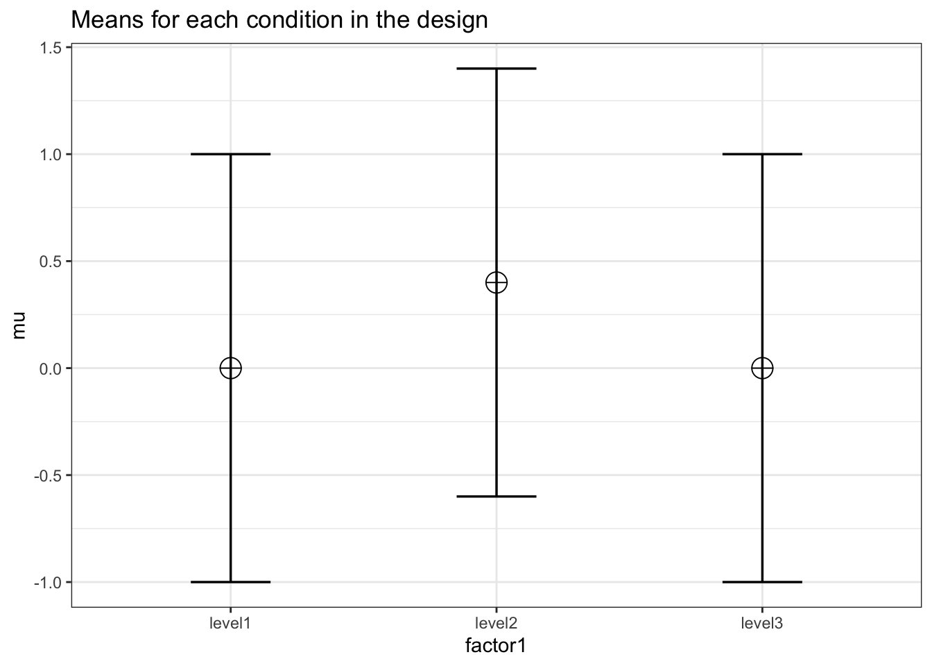
K <- 3
mu <- c(0, 0.4, 0.0)
n <- 145
sd <- 1
r <- 0
design = paste(K, "b", sep = "")

design_result <- ANOVA_design(
  design = design,
  n = n,
  mu = mu,
  sd = sd,
  labelnames = c("factor1", "level1", "level2", "level3")
  )

simulation_result <- ANOVA_power(design_result, 
                                 alpha_level = alpha_level, 
                                 nsims = nsims,
                                 verbose = FALSE)

Table 15.6: Simulated ANOVA Result

	power	effect_size
anova_factor1	94.75	0.0386366

exact_result <- ANOVA_exact(design_result,
                            alpha_level = alpha_level,
                            verbose = FALSE)

Table 15.7: Exact ANOVA Result

	power	partial_eta_squared	cohen_f	non_centrality
factor1	94.89169	0.034565	0.1892154	15.46667

15.7.4 Variation 2

# give sample sizes (all samples sizes are equal)
N = 82
# give effect size d
d1 = .4 #difference between the extremes
d2 = .2 #third condition goes with the highest extreme
# give number of simulations
nSim = nsims
# give alpha levels
#alpha level for the omnibus ANOVA
alpha1 = .05 
#alpha level for three post hoc one-tail t-test Bonferroni correction
alpha2 = .05 

# create vectors to store p-values
p1 <- numeric(nSim) #p-value omnibus ANOVA
p2 <- numeric(nSim) #p-value first post hoc test
p3 <- numeric(nSim) #p-value second post hoc test
p4 <- numeric(nSim) #p-value third post hoc test
pes1 <- numeric(nSim) #partial eta-squared

for (i in 1:nSim) {
#for each simulated experiment

x <- rnorm(n = N, mean = 0, sd = 1)
y <- rnorm(n = N, mean = d1, sd = 1)
z <- rnorm(n = N, mean = d2, sd = 1)
data = c(x, y, z)
groups = factor(rep(letters[24:26], each = N))
test <- aov(data ~ groups)
pes1[i] <- etaSquared(test)[1, 2]
p1[i] <- summary(test)[[1]][["Pr(>F)"]][[1]]
p2[i] <- t.test(x, y)$p.value
p3[i] <- t.test(x, z)$p.value
p4[i] <- t.test(y, z)$p.value
data = c(x, y)
groups = factor(rep(letters[24:25], each = N))
test <- aov(data ~ groups)
pes2[i] <- etaSquared(test)[1, 2]
}

sum(p1 < alpha1) / nSim
sum(p2 < alpha2) / nSim
sum(p3 < alpha2) / nSim
sum(p4 < alpha2) / nSim
mean(pes1)
mean(pes2)

15.7.5 Three conditions replication

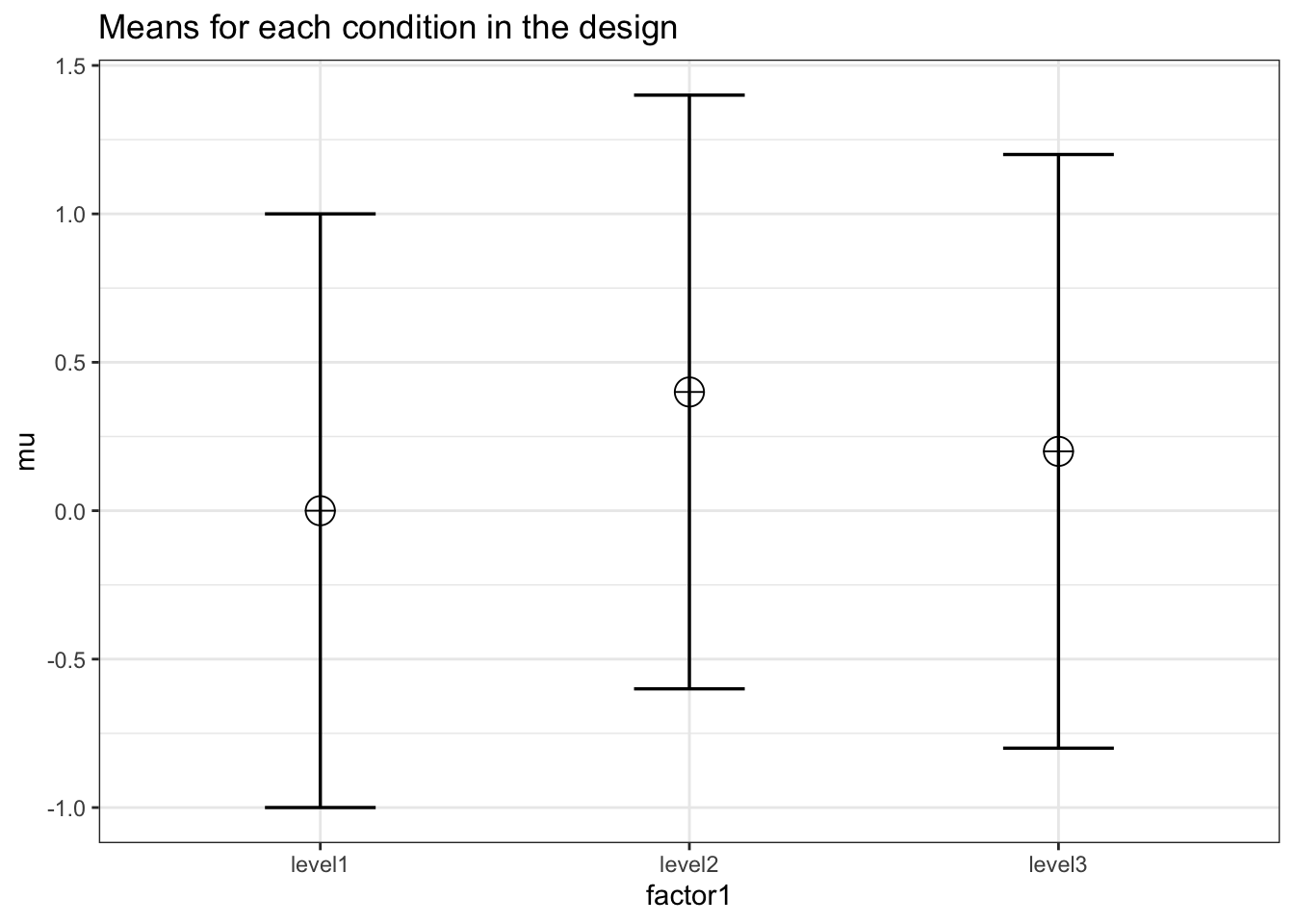
K <- 3
mu <- c(0, 0.4, 0.2)
n <- 82
sd <- 1
design = paste(K, "b", sep = "")

design_result <- ANOVA_design(
  design = design,
  n = n,
  mu = mu,
  sd = sd,
  labelnames = c("factor1", "level1", "level2", "level3")
  )

simulation_result <- ANOVA_power(design_result, 
                                 alpha_level = alpha_level, 
                                 nsims = nsims,
                                 verbose = FALSE)

Table 15.8: Simulated ANOVA Result

	power	effect_size
anova_factor1	62.9	0.0340814

exact_result <- ANOVA_exact(design_result,
                            alpha_level = alpha_level,
                            verbose = FALSE)

Table 15.9: Exact ANOVA Result

	power	partial_eta_squared	cohen_f	non_centrality
factor1	61.94317	0.0262863	0.1643042	6.56

15.8 Repeated Measures

We can reproduce the same results as Brysbaert finds with his code:

design <- "3w"
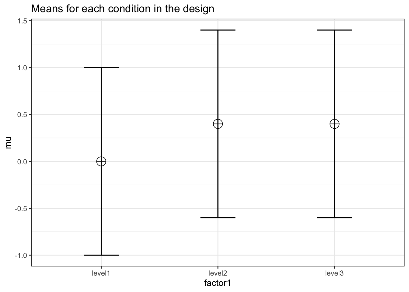
n <- 75
mu <- c(0, 0.4, 0.4)
sd <- 1
r <- 0.5
labelnames <- c("speed", "fast", "medium", "slow")

We create the within design, and run the simulation

design_result <- ANOVA_design(design = design,
                   n = n, 
                   mu = mu, 
                   sd = sd, 
                   r = r, 
                   labelnames = labelnames)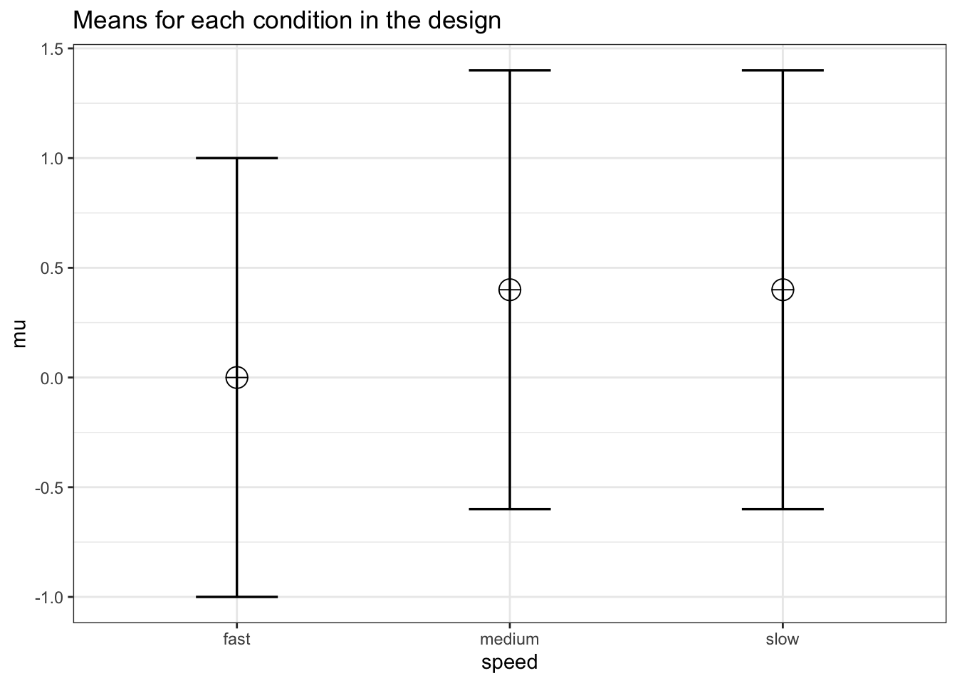

simulation_result <- ANOVA_power(design_result, 
                                 alpha_level = alpha_level, 
                                 nsims = nsims,
                                 verbose = FALSE)

Table 15.10: Simulated ANOVA Result

	power	effect_size
anova_speed	95.11	0.1070021

exact_result <- ANOVA_exact(design_result,
                            alpha_level = alpha_level,
                            verbose = FALSE)

Table 15.11: Exact ANOVA Result

	power	partial_eta_squared	cohen_f	non_centrality
speed	95.29217	0.097561	0.328798	16

Results

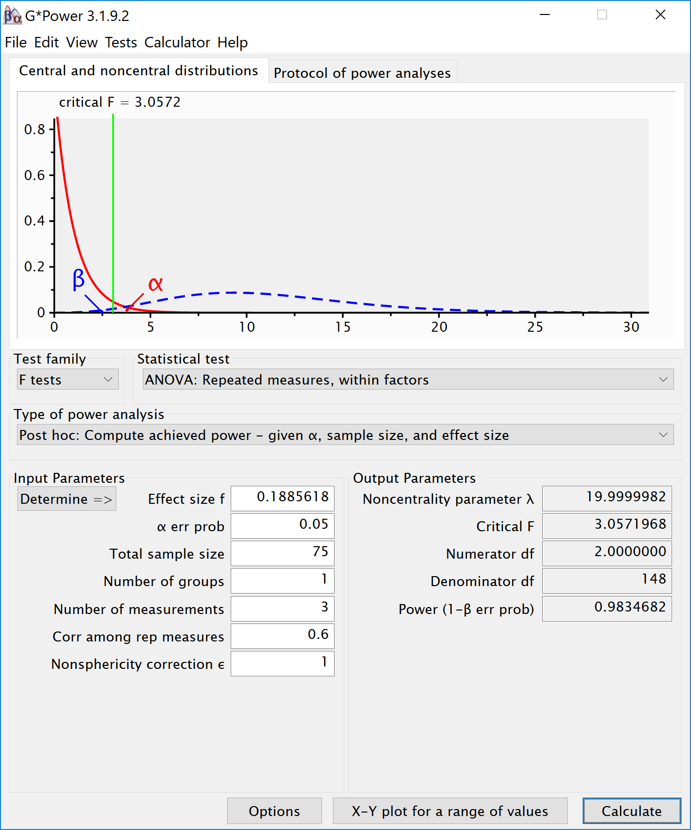
The results of the simulation are very similar. Power for the ANOVA F-test is around 95.2%. For the three paired t-tests, power is around 92.7. This is in line with the a-priori power analysis when using Gpower:

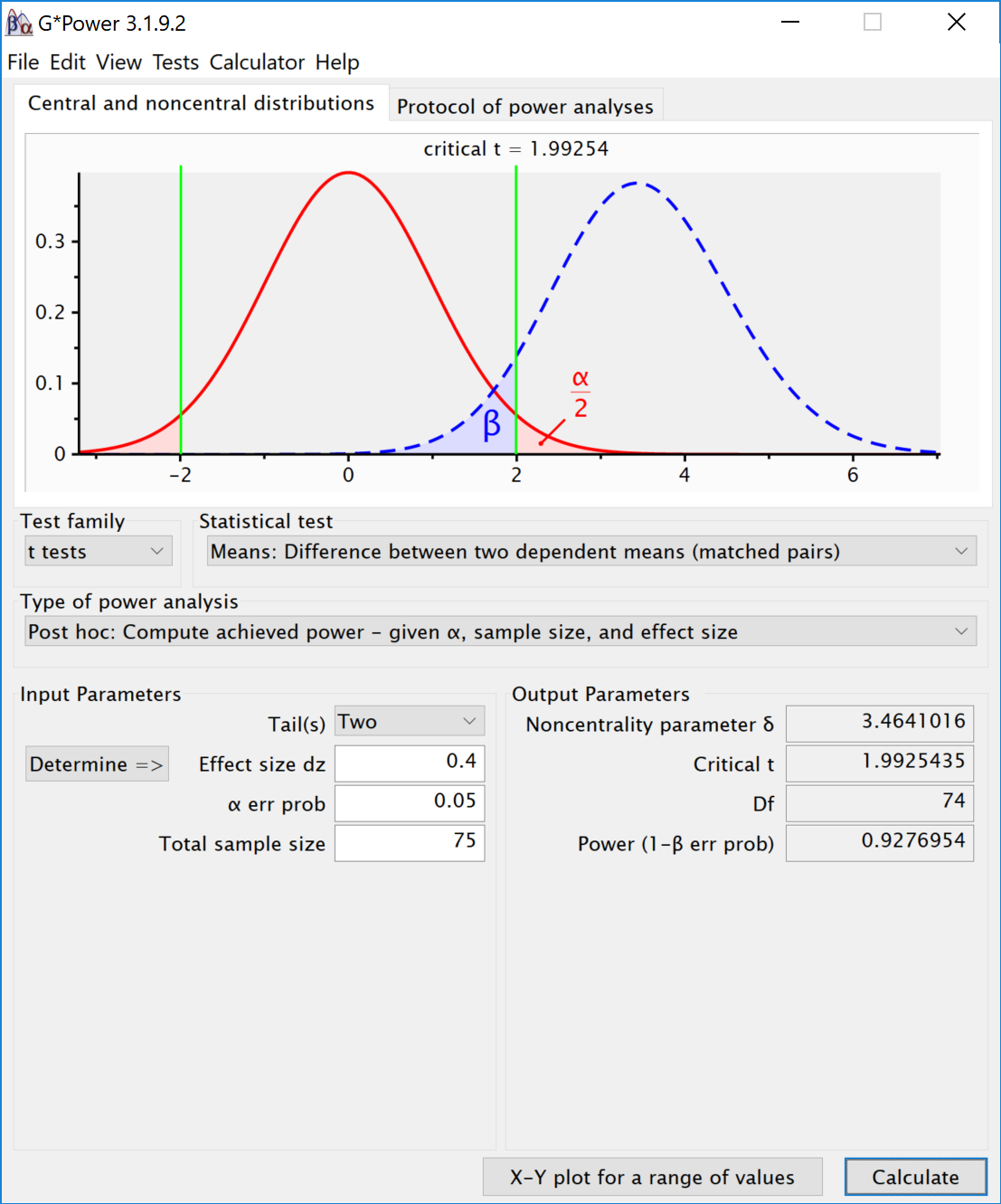
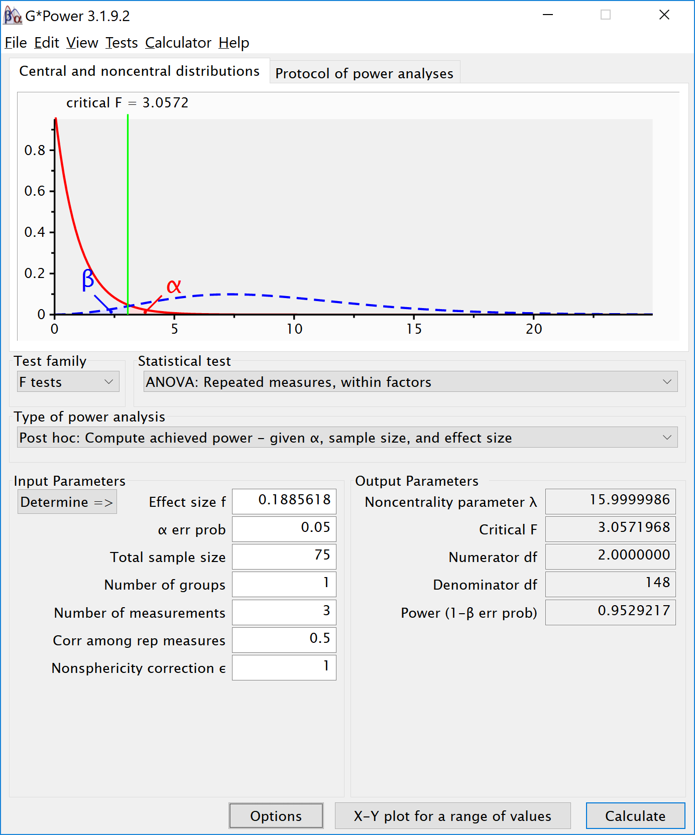
We can perform an post-hoc power analysis in Gpower. We can calculate Cohen´s f based on the means and sd, using our own custom formula.

# Our simulation is based onthe following means and sd:
# mu <- c(0, 0.4, 0.4)
# sd <- 1
# Cohen, 1988, formula 8.2.1 and 8.2.2
f <- sqrt(sum((mu - mean(mu)) ^ 2) / length(mu)) / sd 

# We can see why f = 0.5*d.
# Imagine 2 group, mu = 1 and 2
# Grand mean is 1.5, 
# we have sqrt(sum(0.5^2 + 0.5^2)/2), or sqrt(0.5/2), = 0.5.
# For Cohen's d we use the difference, 2-1 = 1. 

The Cohen´s f is 0.1885618. We can enter the f (using the default ’as in G*Power 3.0’ in the option window) and enter a sample size of 75, number of groups as 1, number of measurements as 3, correlation as 0.5. This yields:

15.8.1 Reproducing Brysbaert Variation 1: Changing Correlation

# give sample size
N = 75
# give effect size d
d1 = .4 #difference between the extremes
d2 = .4 #third condition goes with the highest extreme
# give the correlation between the conditions
r = .6 #increased correlation
# give number of simulations
nSim = nsims
# give alpha levels
alpha1 = .05 #alpha level for the omnibus ANOVA
alpha2 = .05 #also adjusted from original by DL

# create vectors to store p-values
p1 <- numeric(nSim) #p-value omnibus ANOVA
p2 <- numeric(nSim) #p-value first post hoc test
p3 <- numeric(nSim) #p-value second post hoc test
p4 <- numeric(nSim) #p-value third post hoc test

# define correlation matrix
rho <- cbind(c(1, r, r), c(r, 1, r), c(r, r, 1))
# define participant codes
part <- paste("part",seq(1:N))
for (i in 1:nSim) {
  
  #for each simulated experiment

  data = mvrnorm(n = N,
  mu = c(0, 0, 0),
  Sigma = rho)
  data[, 2] = data[, 2] + d1
  data[, 3] = data[, 3] + d2
  datalong = c(data[, 1], data[, 2], data[, 3])
  conds = factor(rep(letters[24:26], each = N))
  partID = factor(rep(part, times = 3))
  output <- data.frame(partID, conds, datalong)
  test <- aov(datalong ~ conds + Error(partID / conds), 
              data = output)
  tests <- (summary(test))
  p1[i] <- tests$'Error: partID:conds'[[1]]$'Pr(>F)'[[1]]
  p2[i] <- t.test(data[, 1], data[, 2], paired = TRUE)$p.value
  p3[i] <- t.test(data[, 1], data[, 3], paired = TRUE)$p.value
  p4[i] <- t.test(data[, 2], data[, 3], paired = TRUE)$p.value
}

sum(p1 < alpha1) / nSim
sum(p2 < alpha2) / nSim
sum(p3 < alpha2) / nSim
sum(p4 < alpha2) / nSim

## [1] 0.9479

## [1] 0.9201

## [1] 0.0494

## [1] 0.9217

design <- "3w"
n <- 75
mu <- c(0, 0.4, 0.4)
sd <- 1
r <- 0.6
labelnames <- c("SPEED", 
                "fast", "medium", "slow")

We create the 3-level repeated measures design, and run the simulation.

design_result <- ANOVA_design(design = design,
                   n = n, 
                   mu = mu, 
                   sd = sd, 
                   r = r, 
                   labelnames = labelnames)

simulation_result <- ANOVA_power(design_result, 
                                 alpha_level = alpha_level, 
                                 nsims = nsims,
                                 verbose = FALSE)

Table 15.12: Simulated ANOVA Result

	power	effect_size
anova_SPEED	98.39	0.1285941

exact_result <- ANOVA_exact(design_result,
                            alpha_level = alpha_level,
                            verbose = FALSE)

Table 15.13: Exact ANOVA Result

	power	partial_eta_squared	cohen_f	non_centrality
SPEED	98.34682	0.1190476	0.3676073	20

Again, this is similar to GPower for the ANOVA:

References

Brysbaert, Marc. 2019. “How Many Participants Do We Have to Include in Properly Powered Experiments? A Tutorial of Power Analysis with Reference Tables.” Journal of Cognition 2 (1). http://doi.org/10.5334/joc.72.