Chapter 11 Power Curve
Power is calculated for a specific value of an effect size, alpha level, and sample size. Because you often do not know the true effect size, it often makes more sense to think of the power curve as a function of the size of the effect. Although power curves could be constructed from Monte Carlo simulations (ANOVA_power) the plot_power function utilizes the ANOVA_exact function within its code because these “exact” simulations are much faster. The basic approach is to calculate power for a specific pattern of means, a specific effect size, a given alpha level, and a specific pattern of correlations. This is one example:
#2x2 design

design_result <- ANOVA_design(design = "2w*2w",
                              n = 20,
                              mu = c(0,0,0,0.5),
                              sd = 1,
                              r = 0.5)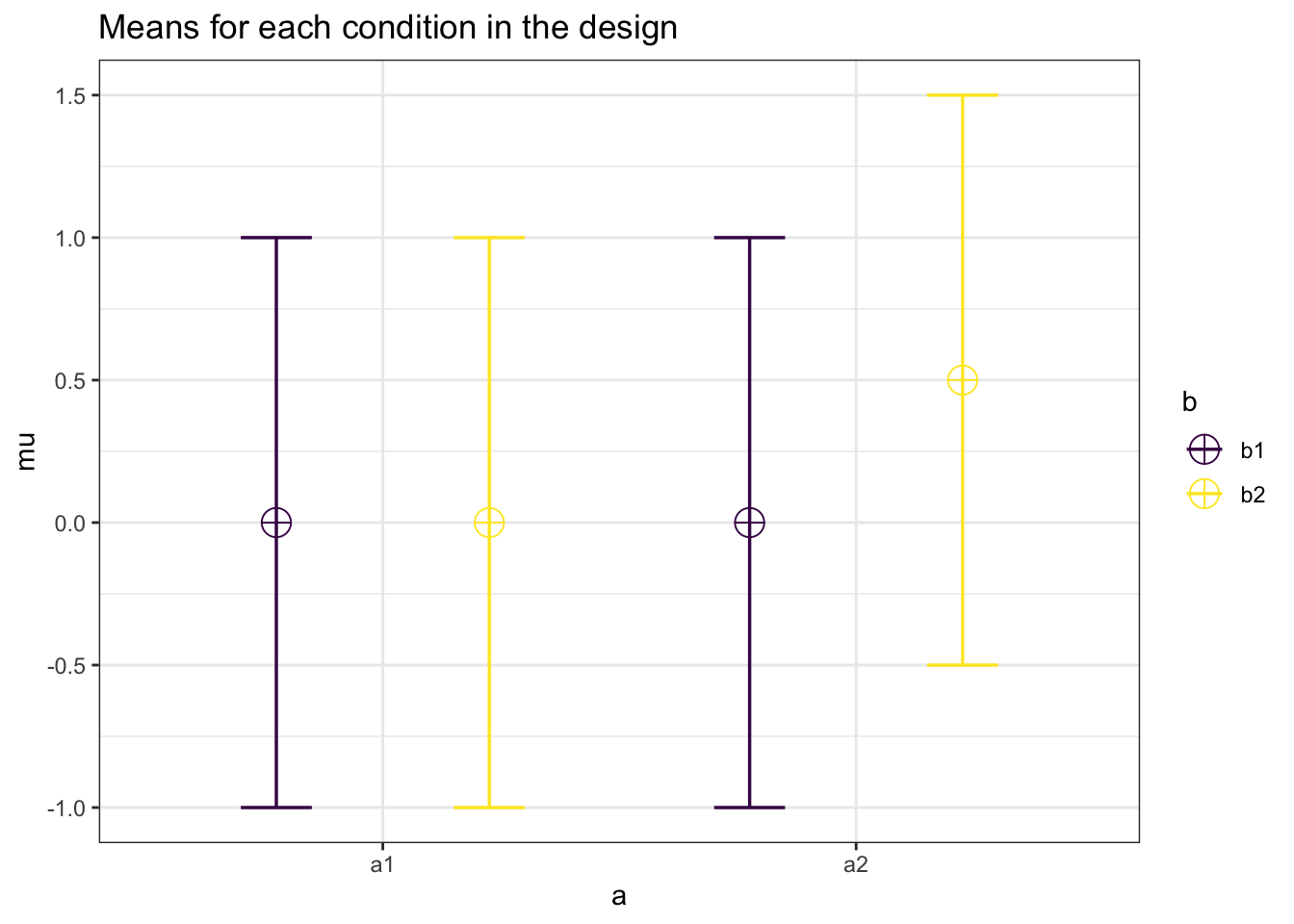
exact_result <- ANOVA_exact(design_result,
                            alpha_level = alpha_level,
verbose = FALSE)| power | partial_eta_squared | cohen_f | non_centrality | |
|---|---|---|---|---|
| a | 32.35926 | 0.1162791 | 0.3627381 | 2.5 |
| b | 32.35926 | 0.1162791 | 0.3627381 | 2.5 |
| a:b | 32.35926 | 0.1162791 | 0.3627381 | 2.5 |
We can make these calculations for a range of sample sizes, to get a power curve. We created a simple function that performs these calculations across a range of sample sizes (from n = 3 to max_, a variable you can specify in the function).
p_a <- plot_power(design_result,
                  max_n = 50,
                  plot = TRUE,
                  verbose = TRUE)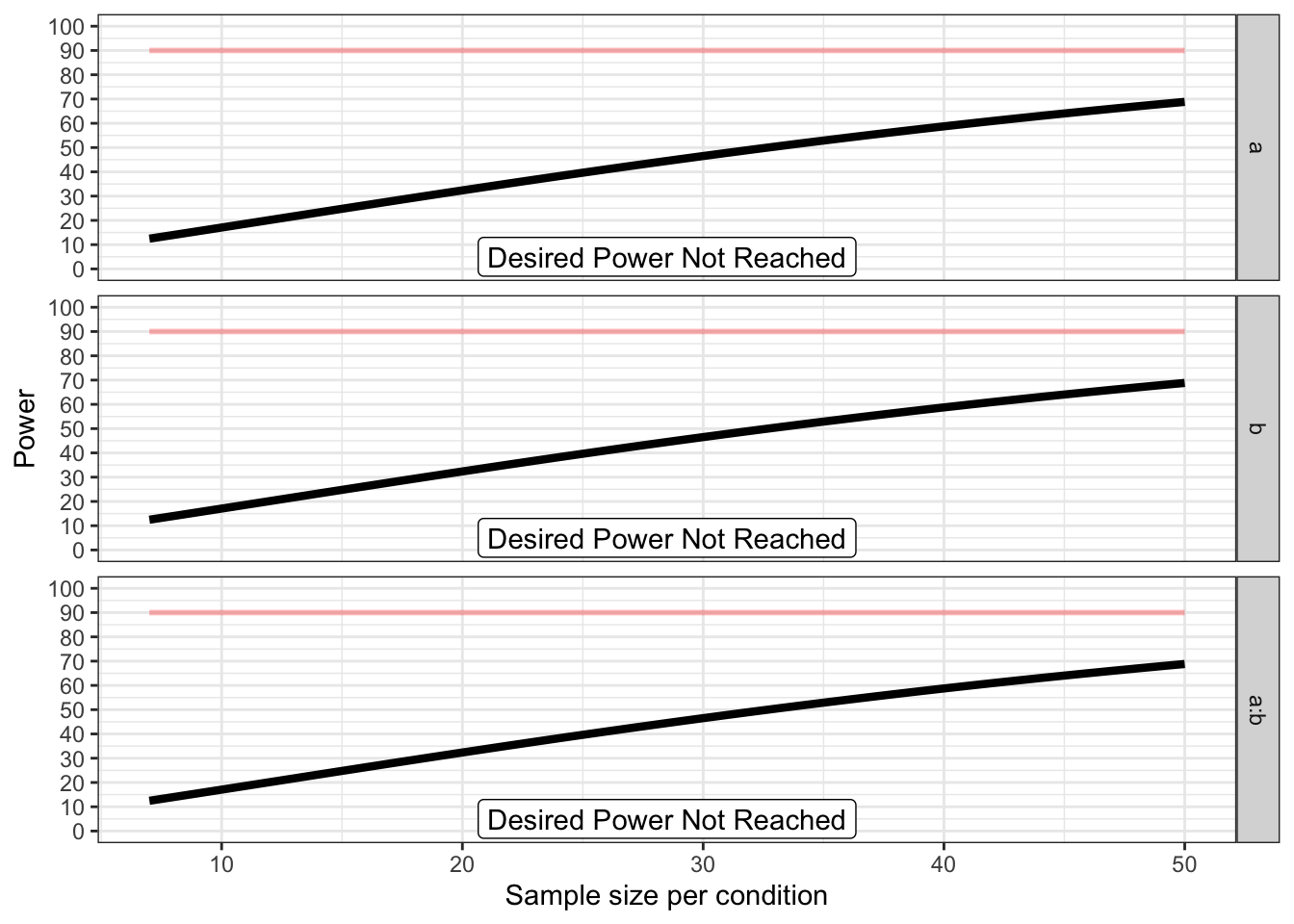
## Achieved Power and Sample Size for ANOVA-level effects
##   variable                     label  n achieved_power desired_power
## 1        a Desired Power Not Reached 50          68.82            90
## 2        b Desired Power Not Reached 50          68.82            90
## 3      a:b Desired Power Not Reached 50          68.82            90
If we run many of these plot_power functions across small changes in the ANOVA_design we can compile a number of power curves that can be combined into a single plot. We do this below. The code to reproduce these plots can be found on the GitHub repository for this book.
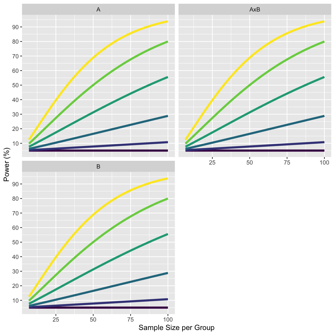
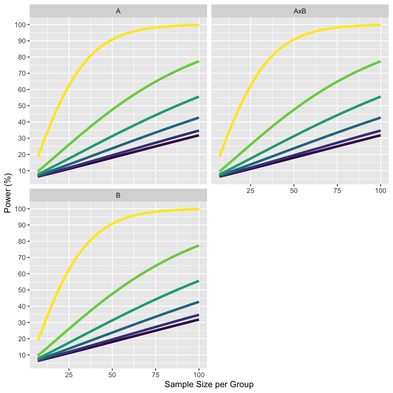
11.1 Explore increase in effect size for moderated interactions.
The design has means 0, 0, 0, 0, with one cell increasing by 0.1, up to 0, 0, 0, 0.5. The standard deviation is set to 1. The correlation between all variables is 0.5.
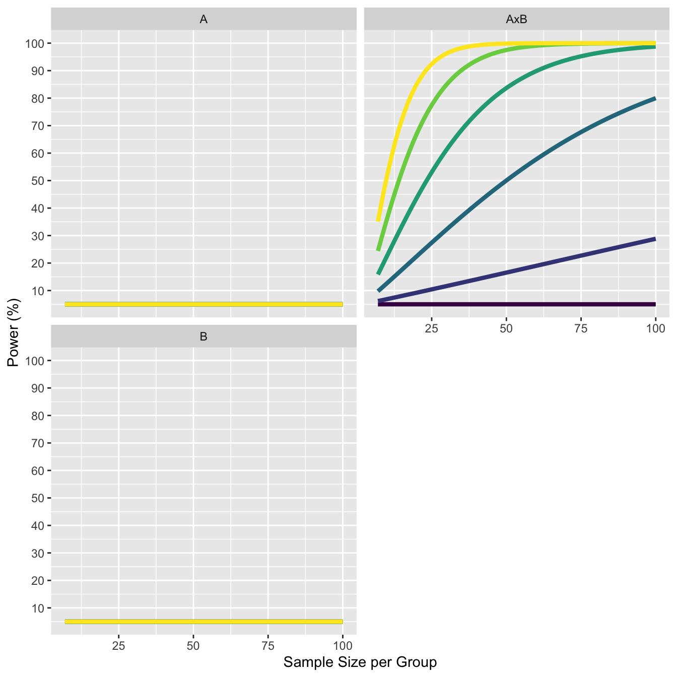
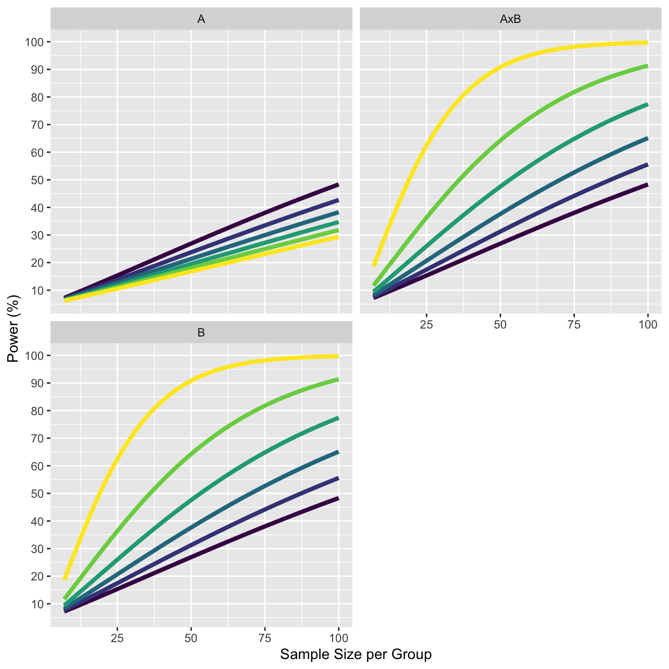
11.2 Explore increase in effect size for cross-over interactions.
The design has means 0, 0, 0, 0, with two cells increasing by 0.1, up to 0.5, 0, 0, 0.5. The standard deviation is set to 1. The correlation between all variables is 0.5.
11.3 Explore increase in correlation in moderated interactions.
The design has means 0, 0, 0, 0.3. The standard deviation is set to 1. The correlation between all variables increases from 0 to 0.9.
11.4 Increasing correlation in on factor decreases power in second factor
As Potvin and Schutz (2000) write:
The more important finding with respect to the effect of r on power relates to the effect of the correlations associated with one factor on the power of the test of the main effect of the other factor. Specifically, if the correlations among the levels of B are larger than those within the AB matrix (i.e., r(B) - r(AB) > 0.0), there is a reduction in the power for the test of the A effect (and the test on B is similarly affected by the A correlations).
We see this in the plots below. As the correlation of the A factor increases from 0.4 to 0.9, we see the power for the main effect decreases.
11.5 Code to Reproduce Power Curve Figures
nsims = 10000
library(Superpower)
library(pwr)
library(tidyverse)
library(viridis)

string <- "2w*2w"
labelnames = c("A", "a1", "a2", "B", "b1", "b2")
design_result <- ANOVA_design(design = string,
                              n = 20,
                              mu = c(0,0,0,0.0),
                              sd = 1,
                              r = 0.5,
                              labelnames = labelnames)
p_a <- plot_power(design_result,
                  max_n = 100)
p_a$power_df$effect <- 0

design_result <- ANOVA_design(design = string,
                              n = 20,
                              mu = c(0,0,0,0.1),
                              sd = 1,
                              r = 0.5,
                              labelnames = labelnames)
p_b <- plot_power(design_result,
                  max_n = 100)

p_b$power_df$effect <- 0.1

design_result <- ANOVA_design(design = string,
                              n = 20,
                              mu = c(0,0,0,0.2),
                              sd = 1,
                              r = 0.5,
                              labelnames = labelnames)
p_c <- plot_power(design_result,
                  max_n = 100)

p_c$power_df$effect <- 0.2

design_result <- ANOVA_design(design = string,
                              n = 20,
                              mu = c(0,0,0,0.3),
                              sd = 1,
                              r = 0.5,
                              labelnames = labelnames)
p_d <- plot_power(design_result,
                  max_n = 100)

p_d$power_df$effect <- 0.3

design_result <- ANOVA_design(design = string,
                              n = 20,
                              mu = c(0,0,0,0.4),
                              sd = 1,
                              r = 0.5,
                              labelnames = labelnames)
p_e <- plot_power(design_result,
                  max_n = 100)

p_e$power_df$effect <- 0.4

design_result <- ANOVA_design(design = string,
                              n = 20,
                              mu = c(0,0,0,0.5),
                              sd = 1,
                              r = 0.5,
                              labelnames = labelnames)
p_f <- plot_power(design_result,
                  max_n = 100)

p_f$power_df$effect <- 0.5


plot_data <- rbind(p_a$power_df, p_b$power_df, p_c$power_df,
                   p_d$power_df, p_e$power_df, p_f$power_df)%>%
  mutate(AxB = `A:B`) %>% select(n,effect,A,B,AxB)

long_data = plot_data %>%
  gather("A", "B", "AxB", key = factor, value = power)

plot1 <- ggplot(long_data, aes(x = n, y = power,
                               color = as.factor(effect))) +
  geom_line(size = 1.5) +
  scale_y_continuous(breaks = seq(0,100,10)) +
  labs(color = "Effect Size",
       x = "Sample Size per Group",
       y = "Power (%)") +
  scale_color_viridis_d() + facet_wrap( ~ factor, ncol=2)

####

design_result <- ANOVA_design(design = string,
                              n = 20,
                              mu = c(0,0,0,0.0),
                              sd = 1,
                              r = 0.5,
                              labelnames = labelnames)
p_a <- plot_power(design_result,
                  max_n = 100)
p_a$power_df$effect <- 0

design_result <- ANOVA_design(design = string,
                              n = 20,
                              mu = c(0.1,0,0,0.1),
                              sd = 1,
                              r = 0.5,
                              labelnames = labelnames)
p_b <- plot_power(design_result,
                  max_n = 100)

p_b$power_df$effect <- 0.1

design_result <- ANOVA_design(design = string,
                              n = 20,
                              mu = c(0.2,0,0,0.2),
                              sd = 1,
                              r = 0.5,
                              labelnames = labelnames)
p_c <- plot_power(design_result,
                  max_n = 100)

p_c$power_df$effect <- 0.2

design_result <- ANOVA_design(design = string,
                              n = 20,
                              mu = c(0.3,0,0,0.3),
                              sd = 1,
                              r = 0.5,
                              labelnames = labelnames)
p_d <- plot_power(design_result,
                  max_n = 100)

p_d$power_df$effect <- 0.3

design_result <- ANOVA_design(design = string,
                              n = 20,
                              mu = c(0.4,0,0,0.4),
                              sd = 1,
                              r = 0.5,
                              labelnames = labelnames)
p_e <- plot_power(design_result,
                  max_n = 100)

p_e$power_df$effect <- 0.4


design_result <- ANOVA_design(design = string,
                              n = 20,
                              mu = c(0.5,0,0,0.5),
                              sd = 1,
                              r = 0.5,
                              labelnames = labelnames)
p_f <- plot_power(design_result,
                  max_n = 100)

p_f$power_df$effect <- 0.5

plot_data <- rbind(p_a$power_df, p_b$power_df, p_c$power_df,
                   p_d$power_df, p_e$power_df, p_f$power_df)%>%
  mutate(AxB = `A:B`) %>% select(n,effect,A,B,AxB)

long_data = plot_data %>%
  gather("A", "B", "AxB", key = factor, value = power)

plot2 <- ggplot(long_data, aes(x = n, y = power,
                               color = as.factor(effect))) +
  geom_line(size = 1.5) +
  scale_y_continuous(breaks = seq(0,100,10)) +
  labs(color = "Effect Size",
       x = "Sample Size per Group",
       y = "Power (%)") +
  scale_color_viridis_d() + facet_wrap( ~ factor, ncol=2)

##

string <- "2w*2w"
labelnames = c("A", "a1", "a2", "B", "b1", "b2")
design_result <- ANOVA_design(design = string,
                              n = 20,
                              mu = c(0,0,0,0.3),
                              sd = 1,
                              r = 0.0,
                              labelnames = labelnames)

p_a <- plot_power(design_result,
                  max_n = 100)

p_a$power_df$correlation <- 0.0


design_result <- ANOVA_design(design = string,
                              n = 20,
                              mu = c(0,0,0,0.3),
                              sd = 1,
                              r = 0.1,
                              labelnames = labelnames)
p_b <- plot_power(design_result,
                  max_n = 100)

p_b$power_df$correlation <- 0.1


design_result <- ANOVA_design(design = string,
                              n = 20,
                              mu = c(0,0,0,0.3),
                              sd = 1,
                              r = 0.3,
                              labelnames = labelnames)
p_c <- plot_power(design_result,
                  max_n = 100)

p_c$power_df$correlation <- 0.3


design_result <- ANOVA_design(design = string,
                              n = 20,
                              mu = c(0,0,0,0.3),
                              sd = 1,
                              r = 0.5,
                              labelnames = labelnames)
p_d <- plot_power(design_result,
                  max_n = 100)

p_d$power_df$correlation <- 0.5


design_result <- ANOVA_design(design = string,
                              n = 20,
                              mu = c(0,0,0,0.3),
                              sd = 1,
                              r = 0.7,
                              labelnames = labelnames)
p_e <- plot_power(design_result,
                  max_n = 100)

p_e$power_df$correlation <- 0.7


design_result <- ANOVA_design(design = string,
                              n = 20,
                              mu = c(0,0,0,0.3),
                              sd = 1,
                              r = 0.9,
                              labelnames = labelnames)
p_f <- plot_power(design_result,
                  max_n = 100)

p_f$power_df$correlation <- 0.9

plot_data <- rbind(p_a$power_df, p_b$power_df,
                   p_c$power_df, p_d$power_df, p_e$power_df, p_f$power_df)%>%
  mutate(AxB = `A:B`) %>% select(n,correlation,A,B,AxB)

long_data = plot_data %>%
  gather("A", "B", "AxB", key = factor, value = power)

plot3 <- ggplot(long_data, aes(x = n, y = power,
                               color = as.factor(correlation))) +
  geom_line(size = 1.5) +
  scale_y_continuous(breaks = seq(0,100,10)) +
  labs(color = "Correlation",
       x = "Sample Size per Group",
       y = "Power (%)") +
  scale_color_viridis_d() + facet_wrap( ~ factor, ncol=2)
##############

string <- "2w*2w"
labelnames = c("A", "a1", "a2", "B", "b1", "b2")
design_result <- ANOVA_design(design = string,
                              n = 20,
                              mu = c(0,0,0,0.3),
                              sd = 1,
                              r <- c(
                                0.4, 0.4, 0.4,
                                0.4, 0.4,
                                0.4),
                              labelnames = labelnames)
p_a <- plot_power(design_result,
                  max_n = 100)

p_a$power_df$corr_diff <- 0

design_result <- ANOVA_design(design = string,
                              n = 20,
                              mu = c(0,0,0,0.3),
                              sd = 1,
                              r <- c(
                                0.5, 0.4, 0.4,
                                0.4, 0.4,
                                0.5),
                              labelnames = labelnames)
p_b <- plot_power(design_result,
                  max_n = 100)

p_b$power_df$corr_diff <- 0.1


design_result <- ANOVA_design(design = string,
                              n = 20,
                              mu = c(0,0,0,0.3),
                              sd = 1,
                              r <- c(
                                0.6, 0.4, 0.4,
                                0.4, 0.4,
                                0.6),
                              labelnames = labelnames)
p_c <- plot_power(design_result,
                  max_n = 100)

p_c$power_df$corr_diff <- 0.2

design_result <- ANOVA_design(design = string,
                              n = 20,
                              mu = c(0,0,0,0.3),
                              sd = 1,
                              r <- c(
                                0.7, 0.4, 0.4,
                                0.4, 0.4,
                                0.7),
                              labelnames = labelnames)
p_d <- plot_power(design_result,
                  max_n = 100)

p_d$power_df$corr_diff <- 0.3

design_result <- ANOVA_design(design = string,
                              n = 20,
                              mu = c(0,0,0,0.3),
                              sd = 1,
                              r <- c(
                                0.8, 0.4, 0.4,
                                0.4, 0.4,
                                0.8),
                              labelnames = labelnames)
p_e <- plot_power(design_result,
                  max_n = 100)

p_e$power_df$corr_diff <- 0.4

design_result <- ANOVA_design(design = string,
                              n = 20,
                              mu = c(0,0,0,0.3),
                              sd = 1,
                              r <- c(
                                0.9, 0.4, 0.4,
                                0.4, 0.4,
                                0.9),
                              labelnames = labelnames)
p_f <- plot_power(design_result,
                  max_n = 100)

p_f$power_df$corr_diff <- 0.5

plot_data <- rbind(p_a$power_df, p_b$power_df, p_c$power_df,
                   p_d$power_df, p_e$power_df, p_f$power_df)%>%
  mutate(AxB = `A:B`) %>% select(n,corr_diff,A,B,AxB)

long_data = plot_data %>%
  gather("A", "B", "AxB", key = factor, value = power)

plot4 <- ggplot(long_data, aes(x = n, y = power,
                               color = as.factor(corr_diff))) +
  geom_line(size = 1.5) +
  scale_y_continuous(breaks = seq(0,100,10)) +
  labs(color = "Difference in Correlation",
       x = "Sample Size per Group",
       y = "Power (%)") +
  scale_color_viridis_d() + facet_wrap( ~ factor, ncol=2)