Percent Change, Sympercents, and Ratios

Last Update: 2024-06-04

The physiology literature’s overuse of percentage change is problematic. While well intentioned, this approach is statistically flawed (see T. J. Cole 2000; Curran-Everett and Williams 2015; T. J. Cole and Altman 2017; Kaiser 1989). A key issue is the false symmetry it creates: a 10% weight loss followed by a 10% gain doesn’t equal the original weight.

Researchers likely use percentage change for its intuitive appeal and ease of comparison across studies. Most people would state they intuitively understand that a 5% increase in something is modest and a 25% increase in something is rather large. Additionally, there is the added benefit that different outcomes can be compared on a more universal scale (much like a standardized mean difference, e.g., Cohen’s d), and evidence for treatments/interventions could be synthesized in something like a meta-analysis (Friedrich, Adhikari, and Beyene 2011; Hedges, Gurevitch, and Curtis 1999).

Alternatives exist that avoid the pitfalls of typical percentage change/difference. Let’s explore these options.

Sympercent

I want to present the “sympercent” as T. J. Cole (2000) calls it. In his original paper, T. J. Cole (2000) presents the simple transformation of continuous variables (\(x\)) using the natural logarithm:

\[ log_ex \]

The symmetric percent difference/change (\(s\%\)) can then be calculated by multiplying the log transformed differences/changes by 100.

\[ s\% = 100 \cdot (log(x) -log(y)) \]

The natural log transformation offers variance stabilization, addressing heteroscedasticity concerns. Additionally, it provides intuitive interpretation. For example, in height differences between British adult males (177.3 cm) and females (163.6 cm), the log transformation yields a symmetric difference of 8.04%, aligning with our perception of a modest height difference (T. J. Cole 2000, e.g., \(100 \cdot (log(177.3) - log(163.6)) = 8.04 \space s\%\)).

Pre-post intervention studies often assess changes in biological variables. Instead of percentage change (\(\%change = \frac{post-pre}{pre}\)), sympercents (\(s\% = 100 \cdot (log(post) -log(pre))\)) offer a symmetric alternative with similar interpretation. For instance, a weight loss from 100 kg to 95 kg yields a 5.1 s% sympercent change, comparable to the 5% change, but without the asymmetry issue.

The Ratio

What is often done, and what I often do, is transform the sympercent to a ratio (I’ve also seen this referred to as a “factor” difference). This can be accomplished because the following is true.

\[ log(x) - log(y) = log(\frac{x}{y}) \]

Therefore, the ratio (\(\frac{x}{y}\)) can be obtained by taken by the exponentiation of the log transformed difference.

\[ ratio = e^{log(x)-log(y)} \] To use our example of weight loss earlier, we can the ratio the following way in R.

exp(log(95)-log(100))

[1] 0.95

# to get inverse
1/exp(log(95)-log(100))

[1] 1.052632

We could then interpret the data as showing a reduction in body weight by a factor of 1.05.

The Ratio Percent

Sometimes I’ve seen people use the log transformation but then use the ratio to calculate a percentage. Essentially the producedure is as follows:

\[ ratio\% = 100*e^{log(x)-log(y)}-100 \]

Again, to use the example from before we get about a 5 percent decrease… However, as you can see from the results below the difference is no longer symmetric.

100*exp(log(95)-log(100))-100

[1] -5

# to get inverse
100*1/exp(log(95)-log(100))-100

[1] 5.263158

I think this is less than ideal, but so long as you are explicit in your methods this is fine as descriptive statistic in my view (i.e., it makes the results of log-transformed data/model more interpretable).

Comparing Percentages

Let’s use a quick example to show how well the percent change, sympercent, and ratio percent track with each other.

Let’s use the weight loss study example from before and create a scenario where the average weight at baseline is 100kg with an SD of 10. I created a random sample below and calculated the different percent for each pair of observations

library(tidyverse)
x = rnorm(10,100,10)
y = rnorm(10,100,10)

df = data.frame(
  x,
  y
)

# Percent Change
df$pc = (x-y)/x

# Sympercent
df$sym = log(x)-log(y)

# Ratio Percent
df$rp  = exp(df$sym)-1

df %>% flextable::flextable() %>%  flextable::theme_tron()

x	y	pc	sym	rp
91.97173	114.65641	-0.24664841	-0.22045868	-0.19784922
127.03798	105.04233	0.17314231	0.19012268	0.20939796
97.56966	105.16089	-0.07780316	-0.07492486	-0.07218680
92.70250	102.91963	-0.11021418	-0.10455295	-0.09927290
108.83737	98.95604	0.09078986	0.09517903	0.09985575
111.32794	113.03202	-0.01530676	-0.01519080	-0.01507600
103.40234	98.53781	0.04704471	0.04818730	0.04936718
93.22710	95.15184	-0.02064567	-0.02043544	-0.02022805
96.85504	91.23349	0.05804088	0.05979340	0.06161719
109.55669	97.62742	0.10888676	0.11528377	0.12219184

As we can see in this example, the sympercent closely approximates the percentage change; so does the ratio percent.

My Opinion

The sympercent suggestion by T. J. Cole (2000) is effective and easy to use. It avoids the downsides of traditional percentage difference/change, offering easier interpretation. Notably, the standard error remains on the same scale when reporting sympercent (unlike ratios). While model assumptions should always be checked, many biological/physiological variables are well-suited for this method

Below, I’m going to demonstrate some examples of using this type of analysis. One for a between-subjects design, another for repeated measures design, and lastly for a two-arm pre-post test design.

Examples of Analyses

The Repeated Measures Study

Let’s look at the Tobacco data from R package “PairedData”. To quote the documentation:

This dataset presents 8 paired data corresponding to numbers of lesions caused by two virus preparations inoculated into the two halves of each tobacco leaves.

library(tidyverse)
library(PairedData)
data(Tobacco)

tb = Tobacco %>% 
  janitor::clean_names() %>%
  as_tibble()

tb

# A tibble: 8 × 3
  plant preparation_1 preparation_2
  <fct>         <int>         <int>
1 P5               31            18
2 P6               20            17
3 P7               18            14
4 P3               17            11
5 P1                9            10
6 P4                8             7
7 P8               10             5
8 P2                7             6

Now, let us assume we want to test for the percent change in the number of lesions (change from preparation 1 to 2). We can accomplish this a number of ways with the t.test function.

# treat it as a one-sample problem

t.test(x = log(tb$preparation_2) - log(tb$preparation_1))

    One Sample t-test

data:  log(tb$preparation_2) - log(tb$preparation_1)
t = -3.1127, df = 7, p-value = 0.01702
alternative hypothesis: true mean is not equal to 0
95 percent confidence interval:
 -0.4989167 -0.0681422
sample estimates:
 mean of x 
-0.2835295 

# treat it as paired samples
(t2 = t.test(x = log(tb$preparation_2),
       y = log(tb$preparation_1),
       paired = TRUE))

    Paired t-test

data:  log(tb$preparation_2) and log(tb$preparation_1)
t = -3.1127, df = 7, p-value = 0.01702
alternative hypothesis: true mean difference is not equal to 0
95 percent confidence interval:
 -0.4989167 -0.0681422
sample estimates:
mean difference 
     -0.2835295 

These results, as interpreted using the sympercents approach, indicate a {r} round(unname(t2$estimate)*100,2) s% change from preparation 1 to preparation 2 (preparation 2 has less lesions).

Therefore, we could report the results as the following:

The second prepartion decreased lesions by approximately 28% (p = 0.017, 95% C.I [6.8%, 49.9%]).

Between Subjects Study

Let’s look at the PlantGrowth data. To quote the documentation:

Results from an experiment to compare yields (as measured by dried weight of plants) obtained under a control and two different treatment conditions.

data(PlantGrowth)

pg = PlantGrowth %>% 
  janitor::clean_names() %>%
  as_tibble()

pg

# A tibble: 30 × 2
   weight group
    <dbl> <fct>
 1   4.17 ctrl 
 2   5.58 ctrl 
 3   5.18 ctrl 
 4   6.11 ctrl 
 5   4.5  ctrl 
 6   4.61 ctrl 
 7   5.17 ctrl 
 8   4.53 ctrl 
 9   5.33 ctrl 
10   5.14 ctrl 
# ℹ 20 more rows

Let’s us compare the three groups using a ordinary least squares (OLS) using an Analysis of Variance (ANOVA) and making pairwise comparisons using the estimated marginal means (also called least square means).

model = lm(log(weight) ~ group,
           data = pg)

flextable::as_flextable(model) %>%  flextable::theme_tron()

	Estimate	Standard Error	t value	Pr(>|t|)
(Intercept)	1.610	0.040	40.583	0.0000	***
grouptrt1	-0.083	0.056	-1.483	0.1496
grouptrt2	0.097	0.056	1.726	0.0958	.
Signif. codes: 0 <= '***' < 0.001 < '**' < 0.01 < '*' < 0.05
Residual standard error: 0.1254 on 27 degrees of freedom
Multiple R-squared: 0.2765, Adjusted R-squared: 0.2229
F-statistic: 5.16 on 27 and 2 DF, p-value: 0.0127

model %>% car::Anova() %>% 
  broom::tidy() %>% flextable::flextable() %>%  flextable::theme_tron()

term	sumsq	df	statistic	p.value
group	0.1623884	2	5.160109	0.01265215
Residuals	0.4248443	27

The ANOVA level effect is significant, let us make those pairwise comparisons on the sympercent scale.

library(emmeans)

emmeans(model,
        pairwise ~ group,
        adjust = "tukey")

$emmeans
 group emmean     SE df lower.CL upper.CL
 ctrl    1.61 0.0397 27     1.53     1.69
 trt1    1.53 0.0397 27     1.45     1.61
 trt2    1.71 0.0397 27     1.63     1.79

Results are given on the log (not the response) scale. 
Confidence level used: 0.95 

$contrasts
 contrast    estimate     SE df t.ratio p.value
 ctrl - trt1   0.0832 0.0561 27   1.483  0.3145
 ctrl - trt2  -0.0968 0.0561 27  -1.726  0.2140
 trt1 - trt2  -0.1800 0.0561 27  -3.209  0.0093

Results are given on the log (not the response) scale. 
P value adjustment: tukey method for comparing a family of 3 estimates 

The output from emmeans shows the estimated marginal means and contrasts on the log scale. For the means, this is rather meaningless. However, for the contrasts, this is the sympercent. Notice, that we have a standard error for the sympercent as well.

From these results we could conclude that neither group significantly differed from control with the estimated differences being less than 10%. However, treatment 2 results in an 18% reduction in weight compared to treatment 1.

2-arm pre-post study

For this example, let us use the data from Plotkin et al. (2022) (data is available for download online). We will use the the outcome variable of the countermovment jump (or CMJ)

df_rct = readr::read_csv(here::here(
  "blog",
  "sympercentchange",
  "dataset.csv"
)) %>%
  janitor::clean_names() %>%
  mutate(id = as.factor(code),
         training_grp = case_when(
           group == 0 ~ "LOAD",
           group == 1 ~ "REPS"
         )) %>%
  dplyr::select(id, training_grp, sex, starts_with("cmj"))

Rows: 38 Columns: 31
── Column specification ────────────────────────────────────────────────────────
Delimiter: ","
chr  (1): SEX
dbl (30): CODE, GROUP, RF30_Pre, RF30_Post, RF50_Pre, RF50_Post, RF70_Pre, R...

ℹ Use `spec()` to retrieve the full column specification for this data.
ℹ Specify the column types or set `show_col_types = FALSE` to quiet this message.

head(df_rct)

# A tibble: 6 × 5
  id    training_grp sex   cmj_pre cmj_post
  <fct> <chr>        <chr>   <dbl>    <dbl>
1 1     LOAD         M        42.4     46.2
2 2     REPS         F        41.4     45.7
3 3     REPS         M        53.8     53.6
4 4     REPS         F        38.6     43.7
5 5     LOAD         F        35.3     36.6
6 6     LOAD         F        31.8     37.1

There are many ways the data could be analyzed. However, I’d caution that an analysis of covariance would be the most efficient option. We also have the choice of making the outcome variable the post score or the change score. Personally, I prefer the post score, it makes most sense to me¹.

Let’s build the models real quick. Notice, that at the ANOVA level with type 3 sums of squares, the p-values are equivalent for the change score and post ANCOVA models.

model_post = lm(log(cmj_post)~  training_grp + log(cmj_pre) + sex,
                data = df_rct)

car::Anova(model_post, type = "3") %>% 
  broom::tidy() %>% 
  flextable::as_flextable() %>%  flextable::theme_tron()

term	sumsq	df	statistic	p.value
character	numeric	numeric	numeric	numeric
(Intercept)	0.0	1	1.4	0.3
training_grp	0.0	1	0.0	0.9
log(cmj_pre)	0.8	1	121.0	0.0
sex	0.0	1	0.1	0.8
Residuals	0.2	34
n: 5

model_cng = lm(I(log(cmj_post)-log(cmj_pre))~  training_grp + log(cmj_pre) + sex,
                data = df_rct)

car::Anova(model_cng, type = "3")%>% 
  broom::tidy() %>% 
  flextable::as_flextable() %>%  flextable::theme_tron()

term	sumsq	df	statistic	p.value
character	numeric	numeric	numeric	numeric
(Intercept)	0.0	1	1.4	0.3
training_grp	0.0	1	0.0	0.9
log(cmj_pre)	0.0	1	1.3	0.3
sex	0.0	1	0.1	0.8
Residuals	0.2	34
n: 5

Now, we can make a pairwise comparison using the estimated marginal means. In this case, we will average the effect, like the model, over both male and female participants

emmeans(model_post, pairwise~training_grp)

$emmeans
 training_grp emmean     SE df lower.CL upper.CL
 LOAD           3.73 0.0186 34     3.69     3.77
 REPS           3.73 0.0198 34     3.69     3.77

Results are averaged over the levels of: sex 
Results are given on the log (not the response) scale. 
Confidence level used: 0.95 

$contrasts
 contrast    estimate     SE df t.ratio p.value
 LOAD - REPS  0.00184 0.0263 34   0.070  0.9448

Results are averaged over the levels of: sex 
Results are given on the log (not the response) scale. 

emmeans(model_cng, pairwise~training_grp)

Warning in (function (object, at, cov.reduce = mean, cov.keep = get_emm_option("cov.keep"), : There are unevaluated constants in the response formula
Auto-detection of the response transformation may be incorrect

$emmeans
 training_grp   emmean     SE df lower.CL upper.CL
 LOAD         -0.00322 0.0186 34  -0.0410   0.0346
 REPS         -0.00506 0.0198 34  -0.0453   0.0352

Results are averaged over the levels of: sex 
Results are given on the identity (not the response) scale. 
Confidence level used: 0.95 

$contrasts
 contrast    estimate     SE df t.ratio p.value
 LOAD - REPS  0.00184 0.0263 34   0.070  0.9448

Results are averaged over the levels of: sex 
Note: contrasts are still on the identity scale 

From this we could conclude that the training modalities elicit similar CMJ responses (difference (LOAD - REPS) = 0.18%; p = 0.9448).

We could even perform an equivalence test, let us assume we want equivalence set to 10 s%.

# Confidence interval
confint(pairs(emmeans(model_post, ~ training_grp)))

 contrast    estimate     SE df lower.CL upper.CL
 LOAD - REPS  0.00184 0.0263 34  -0.0517   0.0553

Results are averaged over the levels of: sex 
Results are given on the log (not the response) scale. 
Confidence level used: 0.95 

# p-value
test(pairs(emmeans(model_post, ~ training_grp)),
     delta = .1)

 contrast    estimate     SE df t.ratio p.value
 LOAD - REPS  0.00184 0.0263 34  -3.728  0.0004

Results are averaged over the levels of: sex 
Results are given on the log (not the response) scale. 
Statistics are tests of equivalence with a threshold of 0.1 
P values are left-tailed 

Checking Model Fit

Contrary to some researcher’s beliefs, the log transformation is not magic, and we should not assume that the model fit is ideal.

As with untransformed data, I would inspect your model to ensure that the model’s assumptions are at least tenable.

One quick way to do this in R is with the performance and see packages. I’d say the plots below are not fantastic, but they aren’t horrible either!

library(see)
library(performance)
check_model(model_post)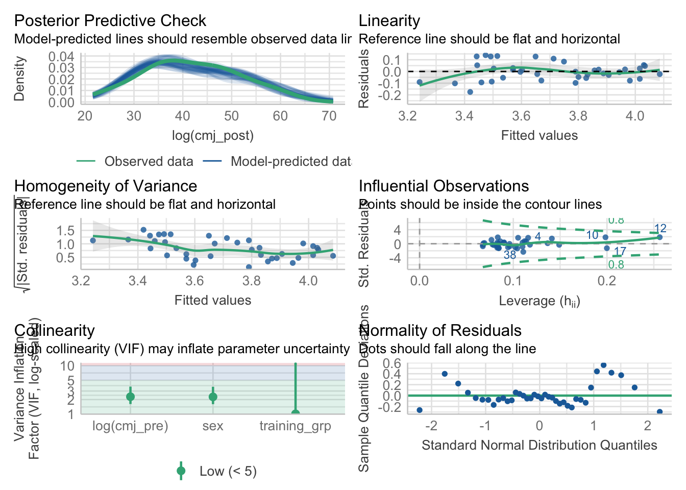

Conclusions

While analyzing data on its original scale is often preferred, presenting results as percentage change can be beneficial for communication and regulatory purposes² In such cases, sympercent is a valuable tool, requiring only a natural log transformation of the raw data, and allowing regression coefficients or contrasts to be interpreted directly as sympercents, thus avoiding the asymmetry issues of traditional percentage change.

References

Cole, T J, and Douglas G Altman. 2017. “Statistics Notes: Percentage Differences, Symmetry, and Natural Logarithms.” BMJ, August, j3683. https://doi.org/10.1136/bmj.j3683.

Cole, T. J. 2000. “Sympercents: Symmetric Percentage Differences on the 100 Loge Scale Simplify the Presentation of Log Transformed Data.” Statistics in Medicine 19 (22): 3109–25. https://doi.org/10.1002/1097-0258(20001130)19:22<3109::aid-sim558>3.0.co;2-f.

Curran-Everett, Douglas, and Calvin L. Williams. 2015. “Explorations in Statistics: The Analysis of Change.” Advances in Physiology Education 39 (2): 49–54. https://doi.org/10.1152/advan.00018.2015.

Friedrich, Jan O., Neill K.J. Adhikari, and Joseph Beyene. 2011. “Ratio of Means for Analyzing Continuous Outcomes in Meta-Analysis Performed as Well as Mean Difference Methods.” Journal of Clinical Epidemiology 64 (5): 556–64. https://doi.org/10.1016/j.jclinepi.2010.09.016.

Hedges, Larry V., Jessica Gurevitch, and Peter S. Curtis. 1999. “THE META-ANALYSIS OF RESPONSE RATIOS IN EXPERIMENTAL ECOLOGY.” Ecology 80 (4): 1150–56. https://doi.org/10.1890/0012-9658(1999)080[1150:tmaorr]2.0.co;2.

Kaiser, Lee. 1989. “Adjusting for Baseline: Change or Percentage Change?” Statistics in Medicine 8 (10): 1183–90. https://doi.org/10.1002/sim.4780081002.

Plotkin, Daniel, Max Coleman, Derrick Van Every, Jaime Maldonado, Douglas Oberlin, Michael Israetel, Jared Feather, Andrew Alto, Andrew D. Vigotsky, and Brad J. Schoenfeld. 2022. “Progressive Overload Without Progressing Load? The Effects of Load or Repetition Progression on Muscular Adaptations.” PeerJ 10 (September): e14142. https://doi.org/10.7717/peerj.14142.

Footnotes

1. I suggest reading Frank Harrell’s blogs/books on this topic https://hbiostat.org/bbr/change#sec-change-gen

2. The FDA suggests that for weight loss drugs the percentage change from baseline should be reported/analyzed. I see no reason why this cannot be the sympercent.