When analyzing ordinal data — like Likert scales, severity ratings, or satisfaction scores— traditional effect sizes often fall short of providing intuitive interpretations. Enter stochastic superiority: a probability-based measure that answers the simple question, “What’s the probability that a randomly selected observation from group A will have a higher outcome than a randomly selected observation from group B?”
In the previous post, I discussed how stochastic superiority could be calculated from predicted probabilities. In this post, we’ll explore how to calculate stochastic superiority for ordinal data using both approximate methods based on model coefficients and exact calculations using predicted probabilities. We’ll demonstrate multiple approaches using R packages like rms, ordinal to the models and emmeans, and marginaleffects to produce the effect size in tersm of stochastic superiority.
What is Stochastic Superiority?
Stochastic superiority, also known as the probability of superiority or concordance probability, is defined mathematically as:
This measure ranges from 0 to 1, where: - 0.5 indicates no difference between groups - Values > 0.5 suggest group A tends to have higher outcomes - Values < 0.5 suggest group A tends to have lower outcomes
Setup and Data
Let’s start by loading our packages and data. We’ll use the wine dataset from the ordinal package, which contains wine ratings on an ordinal scale.
library(rms)library(ordinal)library(emmeans)library(marginaleffects)library(tidyverse)# Load the wine datasetdata(wine)# Quick look at the data structurestr(wine)
First, let’s define our key functions for calculating stochastic superiority.
Fast Stochastic Superiority Calculation
#' Calculate stochastic superiority of group A over group B#' #' @param prob_a Numeric vector of probabilities for group A (in ordinal order)#' @param prob_b Numeric vector of probabilities for group B (in ordinal order) #' @return Numeric value between 0 and 1 representing P(A > B) + 0.5 * P(A = B)stochastic_superiority_fast <-function(prob_a, prob_b) {# Input validationif (length(prob_a) !=length(prob_b)) {stop("prob_a and prob_b must have the same length") } n <-length(prob_a)# Step 1: Create probability matrices a_matrix <-matrix(rep(prob_a, n), nrow = n, byrow =FALSE) # pi_A in columns b_matrix <-matrix(rep(prob_b, n), nrow = n, byrow =TRUE) # pi_B in rows# Step 2: Joint probabilities joint_probs <- a_matrix * b_matrix # Element-wise: pi_{A,i} * pi_{B,j}# Step 3: Weight matrix using row/column indices weights <-ifelse(row(joint_probs) >col(joint_probs), 1, # i > jifelse(row(joint_probs) ==col(joint_probs), 0.5, 0)) # i = j or i < j# Step 4: Sum weighted joint probabilitiesreturn(sum(joint_probs * weights))}
Approximate Stochastic Superiority from Coefficients
We can also approximate stochastic superiority directly from model coefficients using formulas derived by Agresti and others:
#' Calculate Ordinal Superiority Measure (gamma)#' #' This function calculates the ordinal superiority measure gamma = P(y1 > y2; x)#' based on a coefficient β from ordinal regression models with different link functions.#' #' @param beta A numeric value or vector representing the group effect coefficient#' @param link Character string specifying the link function#' @return Numeric value or vector of ordinal superiority measures γordinal_superiority <-function(beta, link ="probit") {# Input validationif (!is.numeric(beta)) {stop("beta must be numeric") } link <-tolower(link) valid_links <-c("probit", "logit", "loglog")if (!link %in% valid_links) {stop("link must be one of: ", paste(valid_links, collapse =", ")) }# Calculate gamma based on link function gamma <-switch(link,"probit"= {pnorm(beta /sqrt(2)) },"logit"= { exp_term <-exp(beta /sqrt(2)) exp_term / (1+ exp_term) },"loglog"= { exp_term <-exp(beta) exp_term / (1+ exp_term) } )return(gamma)}
Model Fitting
Let’s fit ordinal regression models using both rms and ordinal packages with different link functions.
I use both packages because calculating, or really the ability to calculate, stochastic superiority from either package differs.
Method 1: Approximate Stochastic Superiority Using emmeans
The first approach uses emmeans to extract contrasts on the linear predictor scale, then applies the appropriate transformation. Note that emmeans takes the approach of calculating the marginal effect at the mean, so when dealing with models predictions that have issues with non-collapsibility, the average effect and the average effect at the mean will differ.
# Function to calculate stochastic superiority with confidence intervalscalc_stoch_sup_emmeans <-function(model, link_type) {emmeans(model, ~ contact) |>contrast(method ="revpairwise") |>data.frame() |>mutate(stoch_sup =ordinal_superiority(estimate, link = link_type),lower.ci =ordinal_superiority(estimate -qnorm(.975) * SE, link = link_type),upper.ci =ordinal_superiority(estimate +qnorm(.975) * SE, link = link_type) ) |>select(contrast, stoch_sup, lower.ci, upper.ci)}# Calculate for all modelsresults_emmeans <-bind_rows(calc_stoch_sup_emmeans(orm_logit, "logit") |>mutate(model ="ORM Logit"),calc_stoch_sup_emmeans(orm_probit, "probit") |>mutate(model ="ORM Probit"),calc_stoch_sup_emmeans(orm_loglog, "loglog") |>mutate(model ="ORM Log-log"),calc_stoch_sup_emmeans(clm_logit, "logit") |>mutate(model ="CLM Logit"),calc_stoch_sup_emmeans(clm_probit, "probit") |>mutate(model ="CLM Probit"),calc_stoch_sup_emmeans(clm_loglog, "loglog") |>mutate(model ="CLM Log-log"))print(results_emmeans)
  contrast stoch_sup  lower.ci  upper.ci       model
1 yes - no 0.7465538 0.6254424 0.8386096   ORM Logit
2 yes - no 0.7302560 0.6179782 0.8230366  ORM Probit
3 yes - no 0.7026008 0.5636053 0.8120858 ORM Log-log
4 yes - no 0.7465538 0.6034265 0.8507974   CLM Logit
5 yes - no 0.7302560 0.5962606 0.8373180  CLM Probit
6 yes - no 0.7121081 0.5875933 0.8111138 CLM Log-log
Method 2: Exact Calculation Using marginaleffects
The second approach uses predicted probabilities to calculate stochastic superiority:
# A tibble: 6 × 4
  model       emmeans  exact linear_predictor
  <chr>         <dbl>  <dbl>            <dbl>
1 ORM Logit     0.747 NA                0.747
2 ORM Probit    0.730 NA                0.730
3 ORM Log-log   0.703 NA                0.703
4 CLM Logit     0.747  0.708           NA
5 CLM Probit    0.730  0.704           NA
6 CLM Log-log   0.712  0.686           NA
Visualization
Let’s visualize the results to better understand the differences:
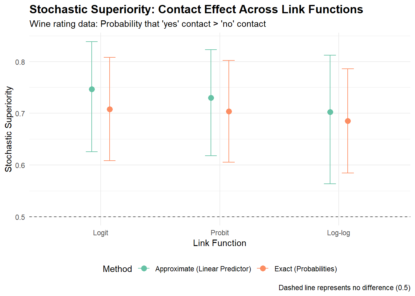
# Prepare data for plottingplot_data <-bind_rows( results_exact |>mutate(method ="Exact (Probabilities)"), results_lp |>mutate(method ="Approximate (Linear Predictor)")) |>separate(model, into =c("package", "link"), sep =" ") |>mutate(link =factor(link, levels =c("Logit", "Probit", "Log-log")),method =factor(method) )ggplot(plot_data, aes(x = link, y = estimate, color = method)) +geom_point(size =3, position =position_dodge(width =0.3)) +geom_errorbar(aes(ymin = conf.low, ymax = conf.high), width =0.2, position =position_dodge(width =0.3)) +geom_hline(yintercept =0.5, linetype ="dashed", alpha =0.7) +scale_color_brewer(type ="qual", palette ="Set2") +labs(title ="Stochastic Superiority: Contact Effect Across Link Functions",subtitle ="Wine rating data: Probability that 'yes' contact > 'no' contact",x ="Link Function",y ="Stochastic Superiority",color ="Method",caption ="Dashed line represents no difference (0.5)" ) +theme_minimal() +theme(plot.title =element_text(size =14, face ="bold"),legend.position ="bottom" )
Comparison of Stochastic Superiority Estimates Across Methods and Link Functions
Key Insights
Based on our analysis, here are the main takeaways:
1. Method Comparison
Exact calculations using predicted probabilities this will work when using marginaleffects with the ordinal package.
Approximate methods using coefficient transformations are computationally faster but may introduce small biases
Both approaches generally yield very similar results for balanced designs
2. Link Function Effects
Different link functions can produce different stochastic superiority estimates
The choice of link function should be based on the underlying data distribution and model fit
Probit and logit links often yield similar results, while log-log can differ more substantially
3. Practical Interpretation
For our wine data, the stochastic superiority of approximately 0.7 means there’s about a 70% probability that a a randomly selected wine with “contact” will receive a higher rating than a randomly selected wine without contact while controlling for serving temperature.
When to Use Each Method?
In the current software environment, you may be limited in choice by what model you choose. My personal preference is the orm function to fit the model and the emmeans package to provide the estimates of interest. However, you might prefer the ordinal package for a variety of reasons due to features listed within that package. What matters is that you realize what each package is capable of and how marginaleffects or emmeans is able to handle the model. Of significant note is that mixed models become much more tricky. To my knowledge, only the ordinal package has support for this in the clmm and clmm2 functions. As of writing this, the marginaleffects package has extremely limited support for either function. The emmeans package has fairly decent support for at least the clmm function. But, then again, you might not want the “marginal effect at the mean” approach that emmeans provides.
Conclusion
Stochastic superiority provides an intuitive, probability-based effect size for ordinal data that’s easy to interpret and communicate. The marginaleffects package offers powerful tools for exact calculation using predicted probabilities, while coefficient-based approximations provide quick alternatives.
The choice between methods depends on your specific needs for accuracy, computational efficiency, and the complexity of your study design. Regardless of the method chosen, stochastic superiority offers a more meaningful interpretation than traditional approaches for ordinal outcomes.