Sometimes as a statistician my job can be repetitive. For many projects, there may be a cluster of variables that all need to be analyzed the same way. For example, we might have a 2 x 3 factorial experiment with 12 outcome variables. A principal investigator may want to have all of them analyzed with an ANOVA, and visualized the same way in a report. Rather than using copy & paste, R can be automated (using a variety of packages) to simplify the process and make the workload (in the long run) lighter.

Data

For simplicity sake, let us use the penguins data from the palmerpenguins R package.

library(palmerpenguins)
data(penguins)

Formatting

Since we are doing a repetitive analysis we then want to make a “tidy” data frame with all the outcome variables. This “long” dataset can be made using the tidyverse set of packages. For this data, we will consider the experimental factors as “species” and “sex”, and consider “island” and “year” as covariates.

library(tidyverse)

── Attaching core tidyverse packages ──────────────────────── tidyverse 2.0.0 ──
✔ dplyr     1.1.4     ✔ readr     2.1.4
✔ forcats   1.0.0     ✔ stringr   1.5.1
✔ ggplot2   3.4.4     ✔ tibble    3.2.1
✔ lubridate 1.9.3     ✔ tidyr     1.3.0
✔ purrr     1.0.2     
── Conflicts ────────────────────────────────────────── tidyverse_conflicts() ──
✖ dplyr::filter() masks stats::filter()
✖ dplyr::lag()    masks stats::lag()
ℹ Use the conflicted package (<http://conflicted.r-lib.org/>) to force all conflicts to become errors

df_pen = penguins %>%
  pivot_longer(cols = c(ends_with(c("mm","g"))), # select outcome variables
               names_to = "variable", # name variables column
               values_to = "y") %>% # name outcomes column 
  mutate(year = as.factor(year)) %>%
  drop_na() # drop missing observations

Now, let us take a peek at the “long” data:

head(df_pen)

# A tibble: 6 × 6
  species island    sex    year  variable               y
  <fct>   <fct>     <fct>  <fct> <chr>              <dbl>
1 Adelie  Torgersen male   2007  bill_length_mm      39.1
2 Adelie  Torgersen male   2007  bill_depth_mm       18.7
3 Adelie  Torgersen male   2007  flipper_length_mm  181  
4 Adelie  Torgersen male   2007  body_mass_g       3750  
5 Adelie  Torgersen female 2007  bill_length_mm      39.5
6 Adelie  Torgersen female 2007  bill_depth_mm       17.4

Analysis

The analysis can then be accomplished with a nested analysis using the purrr R package and its nest function.

# Create nested data sets
df_stats1 = df_pen %>%
  group_by(variable) %>%
  nest()

As you can see the nest function the dataset is now nested by the variable.

df_stats1

# A tibble: 4 × 2
# Groups:   variable [4]
  variable          data              
  <chr>             <list>            
1 bill_length_mm    <tibble [333 × 5]>
2 bill_depth_mm     <tibble [333 × 5]>
3 flipper_length_mm <tibble [333 × 5]>
4 body_mass_g       <tibble [333 × 5]>

Now, let us use mutate to perform our analyses by creating a number of new columns containing the output from the analyses.

For simplicity, let’s assume our request stated that they wanted 1) a ANOVA (type 3 sums of squares) and 2) a visualization of the data. I don’t necessarily recommend such a brief set of output¹

library(rstatix)


Attaching package: 'rstatix'

The following object is masked from 'package:stats':

    filter

# For our ANOVAs
df_stats2 = df_stats1 %>%
  mutate(model = map(data, # build the model
                     ~lm(y ~ species*sex+year+island,
                         data = .)), # dot tells map use "data" column from nested dataset
         anova = map(model, # Get ANOVA table
                     ~car::Anova(., type = "III")),
         aov_summary = map(anova,
                           ~anova_summary(.,effect.size = "pes")),
         plot = map(data, # Plot raw data
                    ~ARCmisc::gg_sum(data = ., # plot data with my bespoke package ;-)
                                     x = species,
                                     y = y,
                                     group = sex,
                                     trace = FALSE,
                                     sum_stat = "med",
                                     show_points = FALSE) + ggprism::theme_prism() +
                      scale_color_viridis_d(end = .8) +
                      scale_fill_viridis_d(end = .8) +
                      labs(y = variable, x = " ") +
                      theme(legend.position = "top")))

Output to a Quarto Document

This part took me a long time to figure out. However, the pander R package, in my opinion, provides the best solution that works across document outputs (in my job I tend to send PDF documents to collaborators).

First, we need to import the pander package, select initial settings, and then create a function for outputting formatted tables.

library(pander)
panderOptions('big.mark', ",")
panderOptions('keep.trailing.zeros',TRUE)
table_fun = function(x, caption = "Table",digits =3){
  
  x = as.data.frame(x) # force into data frame
  if("p" %in% colnames(x)){
    x = x %>%
      mutate(p = scales::pvalue(p)) # format p-values
  }

    
  names(x) = pandoc.strong.return(names(x)) # output column names as bold
  
  pander::pander(
    x,
    caption = caption,
    digits = digits,
    style = "rmarkdown",
    split.tables = 300
  )
}

Now, we can go through a for loop to print the results of every variable in our analysis pipeline.

for (vari1 in unique(df_stats2$variable)){
  # print a header
   pander::pandoc.header(paste0("Analysis: ",vari1),
                         level = 2)
  # filter out other variables
df_stats = df_stats2 %>%
  filter(variable == vari1)

   # ANOVA contents
   pander::pandoc.p(table_fun(subset(df_stats, variable == vari1)$aov_summary[[1]],
             caption = "ANOVA"))
   # adding also empty lines, to be sure that this is valid Markdown
   
   pander::pandoc.p('<br>')
   
   # put plot on separate page if it were a PDF document 
   # # by adding in \newpage latex command

   pander::pandoc.p('\\newpage')
   
   # output plot
   
   plt = subset(df_stats, variable == vari1)$plot[[1]] 
   
   print(plt)
   
   pander::pandoc.p('\\newpage')

}

Analysis: bill_length_mm

ANOVA
Effect	DFn	DFd	F	p	p<.05	pes
species	2	323	261.55	<0.001	*	0.618
sex	1	323	68.56	<0.001	*	0.175
year	2	323	4.49	0.012	*	0.027
island	2	323	1.05	0.351		0.006
species:sex	2	323	2.30	0.102		0.014

Analysis: bill_depth_mm

ANOVA
Effect	DFn	DFd	F	p	p<.05	pes
species	2	323	184.523	<0.001	*	0.533
sex	1	323	111.488	<0.001	*	0.257
year	2	323	1.881	0.154		0.012
island	2	323	1.184	0.307		0.007
species:sex	2	323	0.396	0.674		0.002

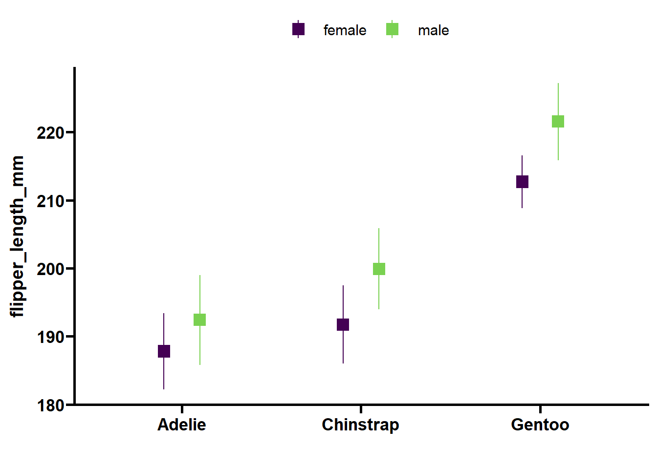
Analysis: flipper_length_mm

ANOVA
Effect	DFn	DFd	F	p	p<.05	pes
species	2	323	273.03	<0.001	*	0.628
sex	1	323	28.72	<0.001	*	0.082
year	2	323	26.50	<0.001	*	0.141
island	2	323	4.18	0.016	*	0.025
species:sex	2	323	5.98	0.003	*	0.036

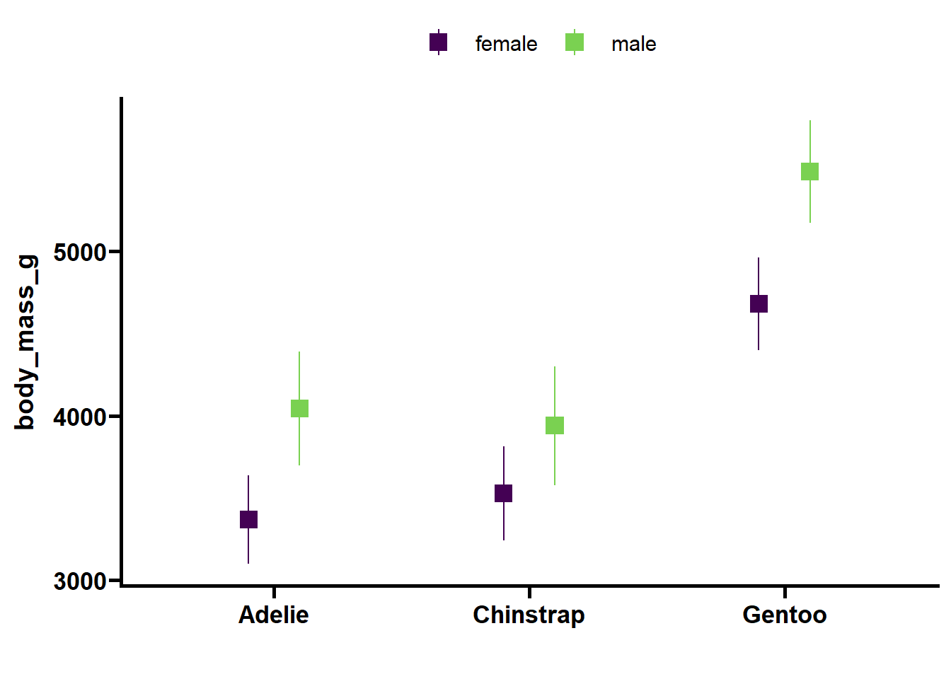
Analysis: body_mass_g

ANOVA
Effect	DFn	DFd	F	p	p<.05	pes
species	2	323	188.498	<0.001	*	5.39e-01
sex	1	323	171.602	<0.001	*	3.47e-01
year	2	323	0.016	0.984		9.73e-05
island	2	323	0.057	0.944		3.54e-04
species:sex	2	323	8.655	<0.001	*	5.10e-02

Conclusion

So, if you are ever in the situation where you have to output the same thing for multiple variables consider using some of this code as a guide. I have used this approach for over a dozen projects now, and to be quite honest I created this post so I had a publicly available version of my code. The code here may seem a bit excessive, but trust me that this will make your life easier as you start to work on the 15th version of analysis report for your collaborator where all they want you to do is change the fontsize on the y-axis for all the plots.

Last Update: 2024-01-31

Footnotes

Often the output is far more extensive and may even vary a little bit based on the variable or possibly issues with the model. Specifically, I often put the output of check_model from easystats in the output to provide a little information on the model diagnostics.↩︎