Introduction to SimplyAgree
Aaron R. Caldwell
Last Updated: 2022-04-27
intro_vignette.RmdThe SimplyAgree R package was created to make the
process of quantifying measurement agreement, consistency, and
reliability. This package expands upon the capabilities of currently
available R packages (such as psych and
blandr) by 1) providing support for agreement studies that
involve multiple observations (agree_test and
agree_reps functions) 2) provide robust tests of agreement
even in simple studies (shieh_test output from the
agree_test function) and 3) a robust set of reliability
statistics (reli_stats function).
In this vignette I will shortly demonstrate the implementation of each function and most of the underlying calculations within each function
Simple Agreement
agree_test
In the simplest scenario, a study may be conducted to compare one
measure (e.g., x) and another (e.g., y). In
this scenario each pair of observations (x and y) are
independent; meaning that each pair represents one
subject/participant. In most cases we have a degree of agreement that we
would deem adequate. This may constitute a hypothesis wherein you may
believe the agreement between two measurements is within a certain limit
(limits of agreement). If this is the goal then the
agree_test function is what you need to use in this
package.
The data for the two measurements are put into the x and
y arguments. If there is a hypothesized limit of agreement
then this can be set with the delta argument (this is
optional). Next, the limit of agreement can be set with the
agree.level and the confidence level (\(1-\alpha\)). Once those are set the
analysis can be run. Please note, this package has pre-loaded data from
the Zou 2013 paper. While data does not conform the assumptions of the
test it can be used to test out many of the functions in this package.
Since there isn’t an a priori hypothesis I will not declare a
delta argument, but I will estimate the 95% confidence
intervals for 80% limits of agreement.
a1 = agree_test(x = reps$x,
                y = reps$y,
                agree.level = .8)
We can then print the general results. These results include the
general parameters of the analysis up top, then the results of the Shieh
exact test for agreement (no conclusion is included due to the lack of a
delta argument being set). Then the limits of agreement,
with confidence limits, are included. Lastly, Lin’s Concordance
Correlation Coefficient, another measure of agreement, is also
included.
print(a1)
#> Limit of Agreement = 80%
#>
#> ###- Shieh Results -###
#> Exact 90% C.I.  [-1.512, 2.3887]
#> Hypothesis Test: No Hypothesis Test
#>
#> ###- Bland-Altman Limits of Agreement (LoA) -###
#>           Estimate Lower CI Upper CI CI Level
#> Bias        0.4383  -0.1669   1.0436     0.95
#> Lower LoA  -1.1214  -1.8039  -0.4388     0.90
#> Upper LoA   1.9980   1.3155   2.6806     0.90
#>
#> ###- Concordance Correlation Coefficient (CCC) -###
#> CCC: 0.4791, 95% C.I. [0.1276, 0.7237]
Next, we can use the generic plot function to produce
visualizations of agreement. This includes the Bland-Altman plot
(type = 1) and a line-of-identity plot
(type = 2).
plot(a1, type = 1)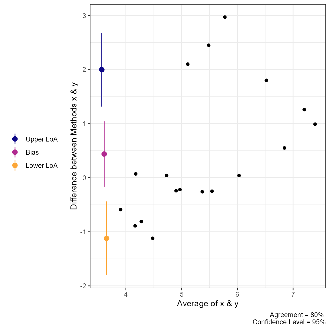
plot(a1, type = 2) 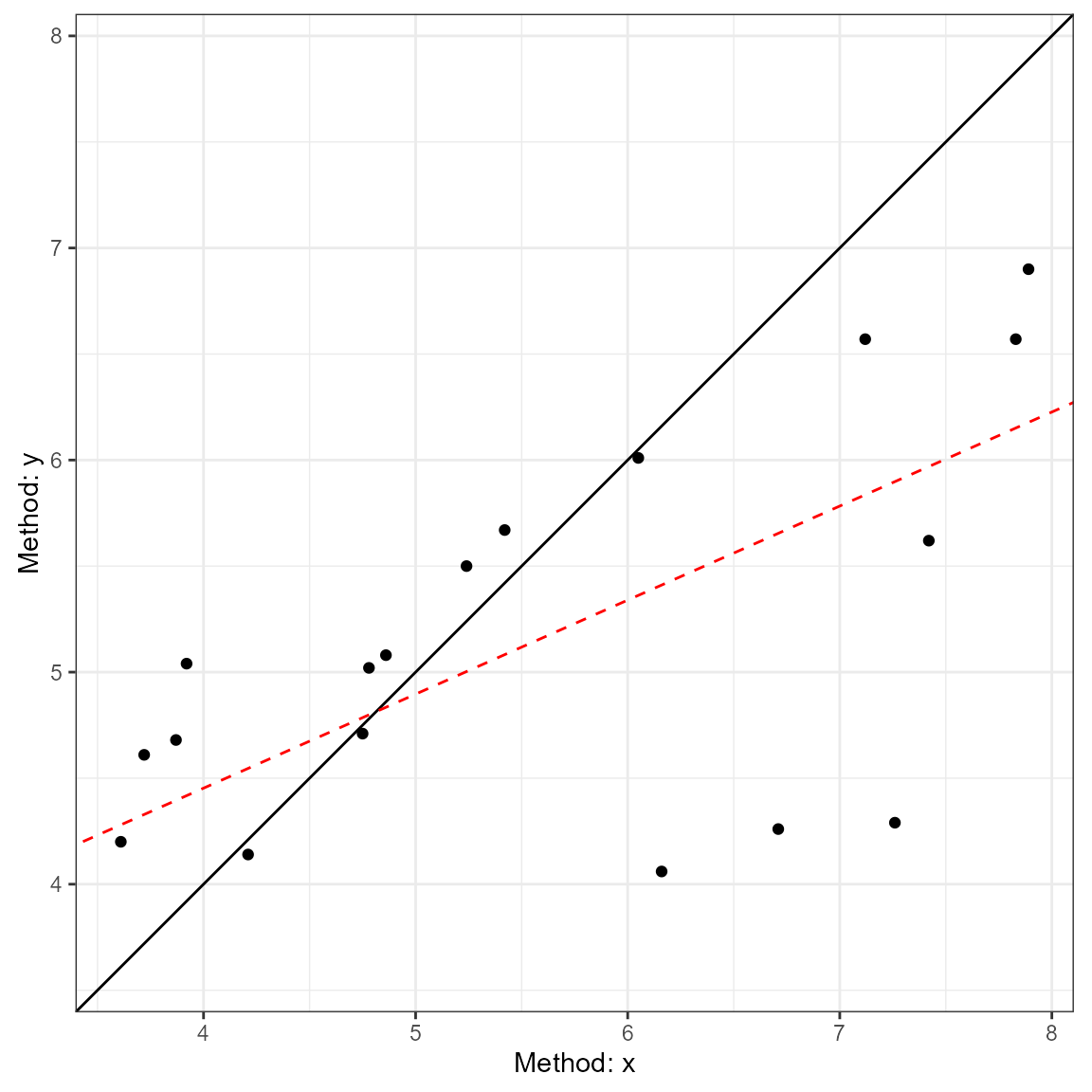
Calculations in agree_test
Shieh’s test
The hypothesis test procedure is based on the “exact” approach details by Shieh (2019). In this procedure the null hypothesis (not acceptable agreement) is rejected if the extreme lower bound and upper bound are within the proposed agreement limits. The agreement limits (\(\hat\theta_{EL} \space and \space \hat\theta_{EU}\)) are calculated as the following:
\[ \hat\theta_{EL,EU} = \bar{d} \pm \gamma_{1-\alpha}\cdot \frac{S}{\sqrt{N}} \]
wherein \(\bar{d}\) is the mean
difference between the two methods, \(S\) is the standard deviation of the
sample, \(N\) is the total number of
pairs, and \(\gamma_{1-\alpha}\)
critical value (which requires a specialized function within
R to estimate).
Limits of Agreement
The reported limits of agreement are derived from the work of Bland and Altman (1986) and Bland and Altman (1999).
\[
LoA = \bar{d} \pm t_{1-\alpha/2,N-1} \cdot
\sqrt{\left[\frac{1}{N}+\frac{(z_{1-\alpha/2})^{2}}{2 \cdot (N-1)}
\right] \cdot S^2}
\] wherein, \(t\) is the
critical t-value at the given sample size and confidence level
(conf.level), \(z\) is the
value of the normal distribution at the given alpha level
(agree.level), and \(S^2\)
is the variance of the difference scores.
Concordance Correlation Coefficient
The CCC was calculated as outlined by Lin (1989) (with later corrections).
\[ \hat\rho_c = \frac{2 \cdot s_{xy}} {s_x^2 + s_y^2+(\bar x-\bar y)^2} \] where \(s_{xy}\) is the covariance, \(s_x^2\) and \(s_y^2\) are the variances of x and y respectively, and \((\bar x-\bar y)\) is the difference in the means of x & y.
Repeated Measures Agreement
In many cases there are multiple measurements taken within subjects
when comparing two measurements tools. In some cases the true underlying
value will not be expected to vary (i.e., replicates;
agree_reps), or multiple measurements may be taken within
an individual and these values are expected to vary (i.e.,
nested design; agree_nest).
The confidence limits on the limits of agreement are based on the
“MOVER” method described in detail by Zou
(2011). However, both functions operate similarly to
agree_test; the only difference being that the data has to
be provided as a data.frame in R.
agree_reps
This function is for cases where the underlying values do not vary within subjects. This can be considered cases where replicate measure may be taken. For example, a researcher may want to compare the performance of two ELISA assays where measurements are taken in duplicate/triplicate.
So, for this function you will have to provide the data frame object
with the data argument and the names of the columns
containing the first (x argument) and second
(y argument) must then be provided. An additional column
indicating the subject identifier (id) must also be
provided. Again, if there is a hypothesized agreement limit then this
could be provided with the delta argument.
a2 = agree_reps(x = "x",
                y = "y",
                id = "id",
                data = reps,
                agree.level = .8)
The results can then be printed. The printing format is very similar
to agree_test, but notice that 1) the hypothesis test is
based on the limits of agreement (MOVER method), 2) the Concordance
Correlation Coefficient is calculated via the U-statistics method, 3)
the Shieh TOST results are missing because they cannot be estimated for
this type of design.
print(a2)
#> Limit of Agreement = 95%
#> Replicate Data Points (true value does not vary)
#>
#> Hypothesis Test: No Hypothesis Test
#>
#> ###- Bland-Altman Limits of Agreement (LoA) -###
#>           Estimate Lower CI Upper CI CI Level
#> Bias        0.7152  -0.6667   2.0971     0.95
#> Lower LoA  -1.2117  -4.7970   0.1054     0.90
#> Upper LoA   2.6421   1.3250   6.2274     0.90
#>
#> ###- Concordance Correlation Coefficient* (CCC) -###
#> CCC: 0.1069, 95% C.I. [-0.1596, 0.3588]
#> *Estimated via U-statistics
plot(a2, type = 1)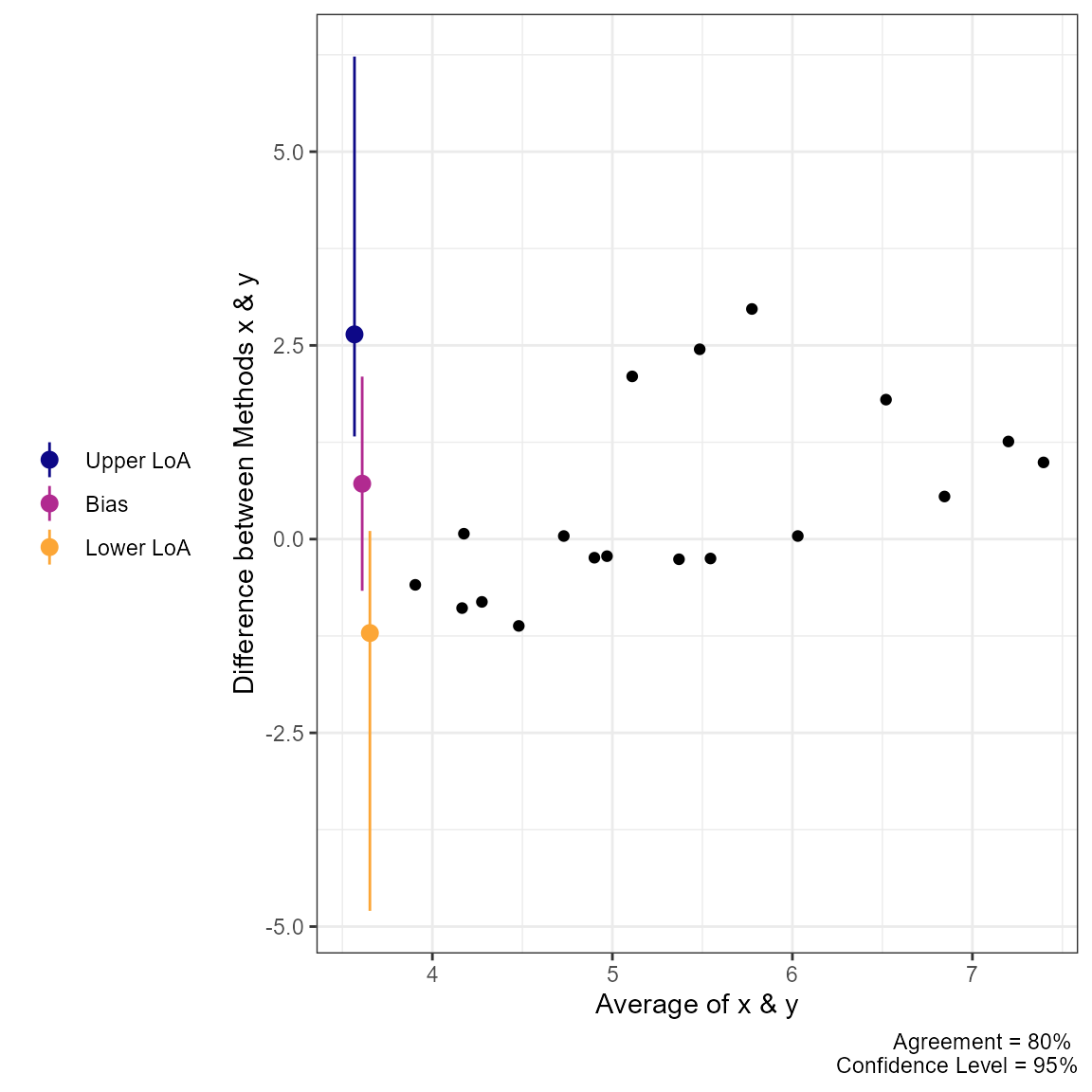
plot(a2, type = 2)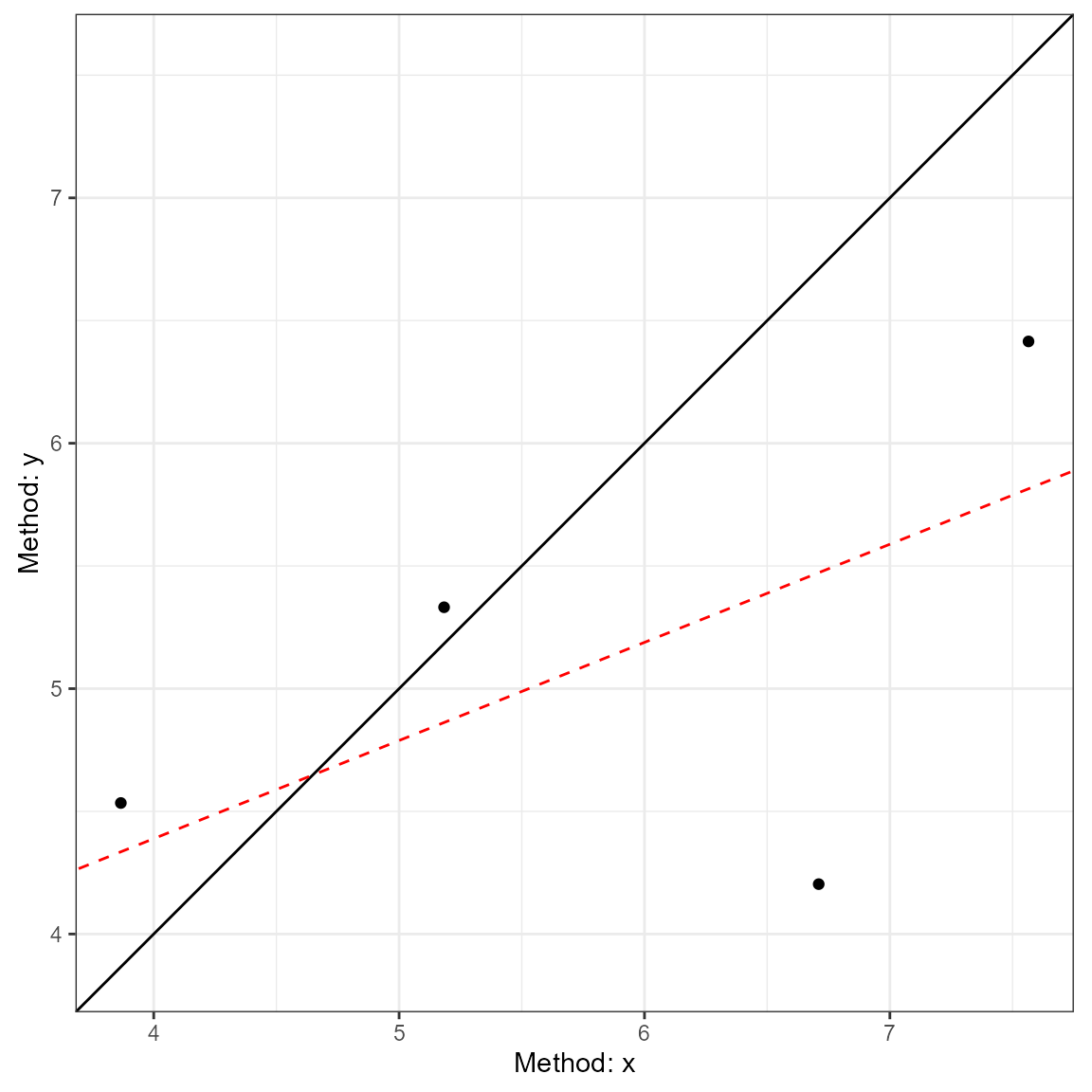
agree_nest
This function is for cases where the underlying values may vary within subjects. This can be considered cases where there are distinct pairs of data wherein data is collected in different times/conditions within each subject. An example would be measuring blood pressure on two different devices on many people at different time points/days.
The function works almost identically to agree_reps but
the underlying calculations are different
a3 = agree_nest(x = "x",
                y = "y",
                id = "id",
                data = reps,
                agree.level = .8)
The printed results (and plots) are very similar to
agree_reps. However, the CCC result now has a warning
because the calculation in this scenario may not be entirely appropriate
given the nature of the data.
print(a3)
#> Limit of Agreement = 95%
#> Nested Data Points (true value may vary)
#>
#> Hypothesis Test: No Hypothesis Test
#>
#> ###- Bland-Altman Limits of Agreement (LoA) -###
#>           Estimate Lower CI Upper CI CI Level
#> Bias        0.7101  -0.6824   2.1026     0.95
#> Lower LoA  -1.1626  -4.8172   0.1811     0.90
#> Upper LoA   2.5828   1.2390   6.2374     0.90
#>
#> ###- Concordance Correlation Coefficient (CCC) -###
#> CCC: 0.4791, 95% C.I. [0.2429, 0.6616]
#> *Estimated via U-statistics; may be biased
plot(a3, type = 1)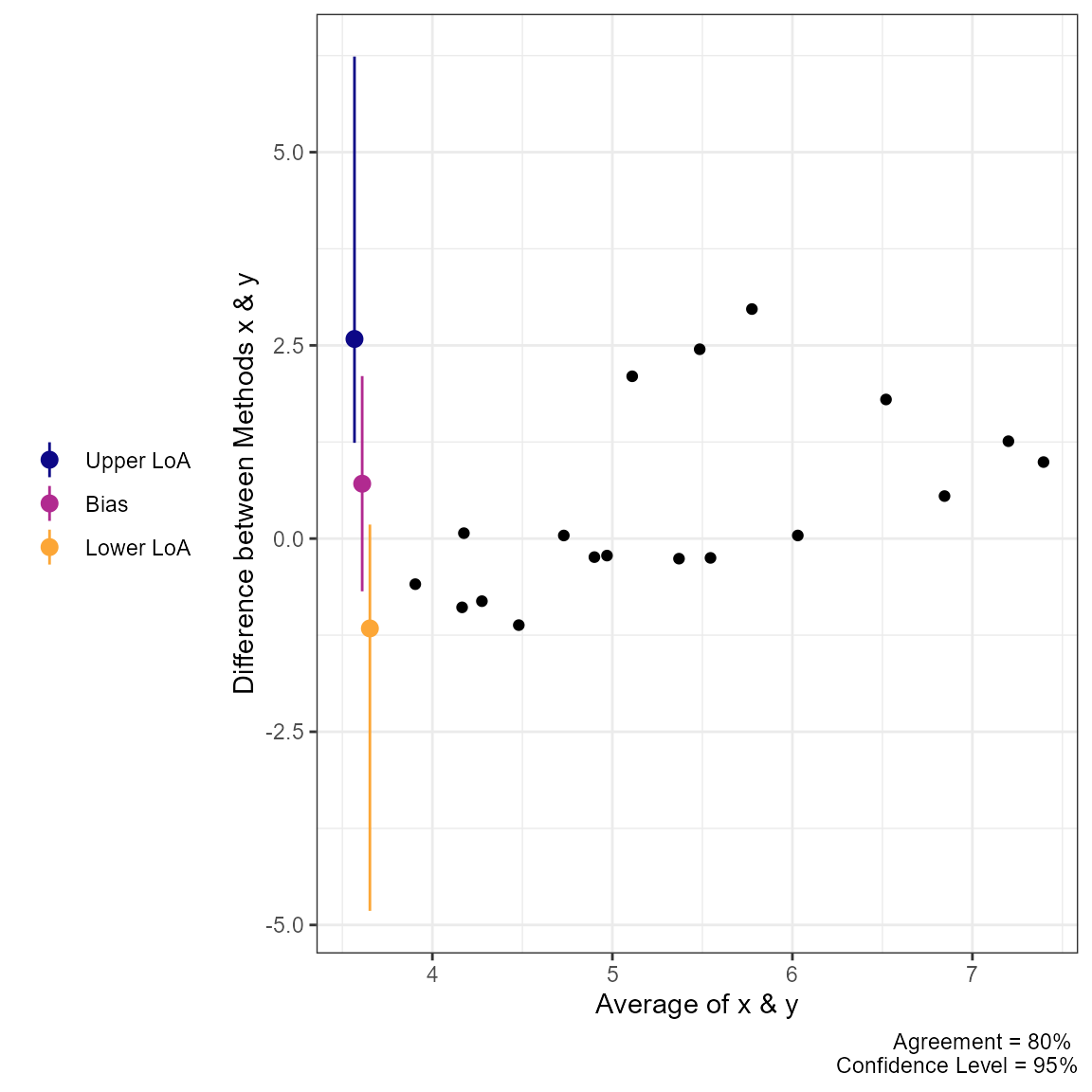
plot(a3, type = 2) ### Calculations for
 agree_reps &
agree_nest
All the calculations for the limits of agreement in these two functions can be found in the article by Zou (2011).
In addition, the CCC calculations are derived from the
cccUst function of the cccrm R package. The
mathematics for this CCC calculation can be found in the work of King, Chinchilli, and Carrasco (2007) and Carrasco, King, and Chinchilli (2009).
Advanced Agreement
In some cases, the agreement calculations involve comparing two methods within individuals within varying conditions. For example, the “recpre_long” data set within this package contains two measurements of rectal temperature in 3 different conditions (where there is a fixed effect of condition). For this particular case we can use bootstrapping to estimate the limits of agreement.
The loa_mixed function can then calculate the limits of
agreement. Like the previous functions, the data set must be set with
the data argument. The diff is the column
which contains the difference between the two measurements. The
condition is the column that indicates the different
conditions that the measurements were taken within. The id
is the column containing the subject/participant identifier. The
plot.xaxis, if utilized, sets the column from which to plot
the data on the x-axis. The final two arguments replicates
and type set the requirements for the bootstrapping
procedure. Warning: This is a computationally heavy
procedure and may take a few minutes to complete. An example code can be
seen below.
a4 = loa_mixed(data = recpre_long,
               diff = "diff",
               condition = "trial_condition",
               id = "id",
               plot.xaxis = "AM",
               replicates = 199,
               type = "perc")
Test-Retest Reliability
Another feature of this R package is the ability to estimate the reliability of a measurement. This R package allows for the calculation of Intraclass Correlation Coefficients (ICC), various standard errors (SEM, SEE, and SEP), and coefficient of variation. All of the underlying calculations (sans the coefficient of variation) is based on the paper by Weir (2005). This is a fairly popular paper within my own field (kinesiology), and hence was the inspiration for creating this function that provides all the calculative approaches included within that manuscript.
For this package, the test-retest reliability statistics can be
calculated with the reli_stats function. This function
allow for data to be input in a long (multiple rows of data for each
subject) or in wide (one row for each subject but a column for each
item/measure).
For the long data form, the column containing the subject identifier
(id), item number (item), and measurements
(measure) are provided. In this function I refer to items
similar to if we were measuring internal consistency for a questionnaire
(which is just a special case of test-retest reliability). So,
item could also be refer to time points, which is what is
typically seen in human performance settings where test-retest
reliability may be evaluated over the course of repeated visits to the
same laboratory. If wide is set to TRUE then
the columns containing the measurements are provided (e.g.,
c("value1","value2","value3")).
To demonstrate the function, I will create a data set in the wide format.
  sf <- matrix(
    c(9,    2,   5,    8,
      6,    1,   3,    2,
      8,    4,   6,    8,
      7,    1,   2,    6,
      10,   5,   6,    9,
      6,   2,   4,    7),
    ncol = 4,
    byrow = TRUE
  )

  colnames(sf) <- paste("J", 1:4, sep = "")
  rownames(sf) <- paste("S", 1:6, sep = "")
  #sf  #example from Shrout and Fleiss (1979)
  dat = as.data.frame(sf)
Now, that we have a data set (dat), I can use it in the
reli_stats function.
test1 = reli_stats(
  data = dat,
  wide = TRUE,
  col.names = c("J1", "J2", "J3", "J4")
)
This function also has generic print and plot functions. The output
from print provides the coefficient of variation, standard errors, and a
table of various intraclass correlation coefficients. Notice the
conclusions about the reliability of the measurement here would vary
greatly based on the statistic being reported. What statistic you should
report is beyond the current vignette, but is heavily detailed in Weir (2005). However, within the table there are
columns for model and measures which describe
the model that is being used and the what these different ICCs are
intended to measure, respectively.
print(test1)
#>
#> Coefficient of Variation (%):  15.36
#> Standard Error of Measurement (SEM):  1.0097
#> Standard Error of the Estimate (SEE):  2.6245
#> Standard Error of Prediction (SEP):  4.065
#>
#> Intraclass Correlation Coefficients
#>            model         measures  type    icc lower.ci upper.ci
#> 1 one-way random        Agreement  ICC1 0.1657 -0.09672   0.6434
#> 2 two-way random        Agreement  ICC2 0.2898  0.04290   0.6911
#> 3  two-way fixed      Consistency  ICC3 0.7148  0.41184   0.9258
#> 4 one-way random   Avg. Agreement ICC1k 0.4428 -0.54504   0.8783
#> 5 two-way random   Avg. Agreement ICC2k 0.6201  0.15204   0.8995
#> 6  two-way fixed Avg. Consistency ICC3k 0.9093  0.73690   0.9804
Also included in the results is a plot of the measurements across the items (e.g., time points).
plot(test1)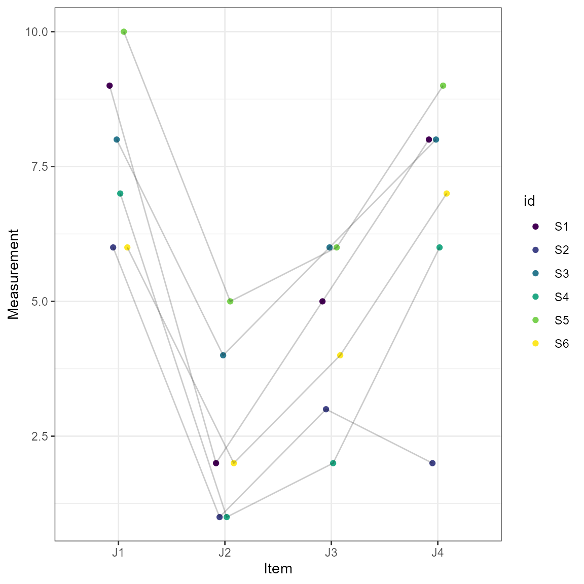
Power Analysis for Agreement
There are surprisingly few resources for planning a study that
attempts to quantify agreement between two methods. Therefore, we have
added one function, with hopefully more in the future, to aid in the
power analysis for simple agreement studies. The current function is
blandPowerCurve which constructs a “curve” of power across
sample sizes, agreement levels, and confidence levels. This is based on
the work of Lu et al. (2016).
For this function the user must define the hypothesized limits of
agreement (delta), mean difference between methods
(mu), and the standard deviation of the difference scores
(SD). There is also the option of adjusting the range of
sample size (default: seq(10,100,1) which is 10 to 100 by
1), the agreement level (default is 95%), and confidence level (default
is 95%). The function then produces a data frame of the results. A quick
look at the head and we can see that we have low statistical power when
the sample size is at the lower end of the range.
power_res <- blandPowerCurve(
  samplesizes = seq(10, 100, 1),
  mu = 0.5,
  SD = 2.5,
  delta = c(6,7),
  conf.level = c(.90,.95),
  agree.level = c(.8,.9)
)

head(power_res)
#>    N  mu  SD delta     power agree.level conf.level
#> 1 10 0.5 2.5     6 0.4870252         0.8        0.9
#> 2 11 0.5 2.5     6 0.5624800         0.8        0.9
#> 3 12 0.5 2.5     6 0.6262736         0.8        0.9
#> 4 13 0.5 2.5     6 0.6802613         0.8        0.9
#> 5 14 0.5 2.5     6 0.7260286         0.8        0.9
#> 6 15 0.5 2.5     6 0.7649104         0.8        0.9
We can then find the sample size at which (or closest to which) a
desired power level with the find_n method for
powerCurve objects created with the function above.
find_n(power_res, power = .8)
#> # A tibble: 8 x 5
#> delta conf.level agree.level power N
#> <dbl> <dbl> <dbl> <dbl> <dbl>
#> 1 6 0.9 0.8 0.798 16
#> 2 6 0.9 0.9 0.802 50
#> 3 6 0.95 0.8 0.798 20
#> 4 6 0.95 0.9 0.802 63
#> 5 7 0.9 0.8 0.847 10
#> 6 7 0.9 0.9 0.800 19
#> 7 7 0.95 0.8 0.775 11
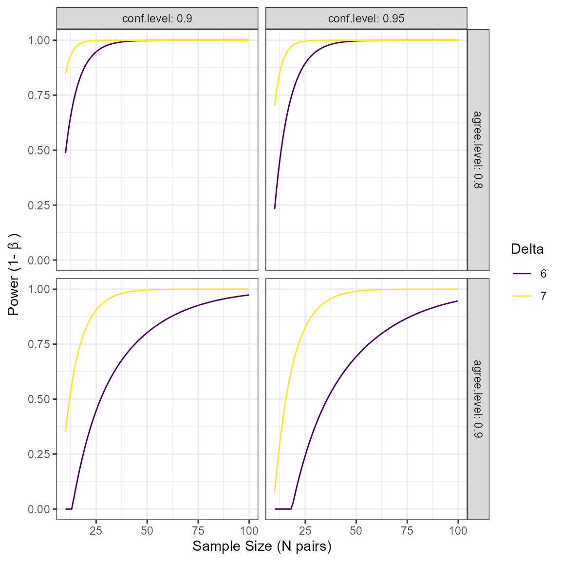
#> 8 7 0.95 0.9 0.806 24Additionally we can plot the power curve to see how power changes
over different levels of delta, agree.level,
and conf.level
plot(power_res)